How not to be engulfed by MAGMA: instructions and model descriptions

library(magma.gsi)
# devtools::load_all()

This document contains the background information for Mark and Age-enhanced Genetic Mixture Analysis (MAGMA) and is organized in three parts: overview descriptions of the MAGMA model, instructions on the latest in the software programs to input data, run the MAGMA model, and summarize results, and detailed descriptions of the MAGMA model and its mathematical theory (the fun stuff).

Overview

MAGMA is a Bayesian genetic stock identification model first developed by the Gene Conservation Lab (GCL) biometrician Jim Jasper. MAGMA is based on the Pella-Masuda model (Pella & Masuda, 2001) and incorporates information on age and hatchery group membership using matched scales and otoliths to allow more detailed stock composition estimates.

Mainly, MAGMA estimates two sets of parameters: population and age. For each mixture (or a stratum), MAGMA estimates a vector of population proportions of wild and hatchery groups. For all mixtures (or all strata) within a year, MAGMA estimates a matrix of age proportions with each row represents a wild or hatchery population. Populations are then combined to represent a reporting group or a fishery stock. An age-by-stock composition, information that is often required for run reconstruction models, is simply the product of age and stock parameters. In a single-stratum example shown below, we can see how the age-by-stock composition is presented. A matrix of made-up age proportions is as follows:

	Age 1	Age 2	Age 3
Stock A	$0.2$	$0.3$	$0.5$
Stock B	$0.4$	$0.5$	$0.1$

The made-up stock proportions are 0.7 and 0.3 for stock A and B in this stratum. Multiplying the age and stock proportions for each stock:

	Age 1	Age 2	Age 3
Stock A	$0.2$	$0.3$	$0.5$	$\times 0.7$
Stock B	$0.4$	$0.5$	$0.1$	$\times 0.3$

The age-by-stock composition¹ for this stratum is:

	Age 1	Age 2	Age 3
Stock A	$0.14$	$0.21$	$0.35$
Stock B	$0.12$	$0.15$	$0.03$

After all age/stock compositions in other strata are calculated in the same fashion, they are multiplied by the harvest proportions of their corresponding strata and summed up to get a weighted average age/stock composition for the whole fishery.

Age proportions are estimated by combining all mixtures/strata within a year, which can be counter-intuitive at the first glance. After all, it may not be reasonable to assume that all mixtures share the same age distribution. However, in the MAGMA model, age compositions are adjusted according to stock proportions for each mixture (i.e., stratum). Because stock proportions are different from mixtures to mixtures, the differences in stock compositions drive the differences in age compositions between mixtures. In the previous example, stock A consists mainly (50%) age 3 fish and is 70% of the total mixture population. Therefore, age 3 fish from stock A is the dominant class in the mixture population. In another stratum, stock B might be the majority of the mixture populations. In which case, we would expect to see that age 2 to be the dominant class because compositions are driven mostly by stock B.

It is not required that all individuals in the data set have an observed genotype or age. Base on data available, MAGMA model assigns a most likely membership for population and/or age to each individual that has unobserved genotype and/or age. However, there should be an adequate sample of genotyped individuals to represent each stratum in the data set. When there is an inadequate number (small or zero sample size) of genotyped individuals in a stratum, MAGMA model estimates population proportions of that stratum based on the overall proportions of all strata combined.

Estimation of age and population compositions in the MAGMA model is done through an algorithm called the Gibbs sampler. The process is initialized by stochastically assigning all individuals with unobserved identities a group membership for population or age class based on specified priors, then the proportions for populations and age classes are “estimated” by drawing values from the full conditional distributions² of the population and age classes. The full conditional distributions are mainly based on numbers of individuals counted in each population and age group. The Gibbs sampler proceeds in the following steps:

1. Determine population memberships of mixture individuals by:

• stochastically assign a (wild) population membership to each individual without observed identity but with genotypes based on its genotypic frequencies and population proportions, and
• stochastically assign a (wild) population membership to each individual without observed identity and without genotypes based on population proportions.

2. If individual’s age is unobserved, assign an age based on the age composition of its assigned population membership.

3. Draw updated values for population and age proportions and baseline allele frequencies from their full conditional distributions based on updates for:

• tallies of individuals in each age class for each population (assigned and observed) for both wild and hatchery groups and
• specified prior values.

This algorithm is repeated until simulations converged to the posterior distribution of the parameters, usually it takes thousands of iterations. We adapted a modified version of the conditional genetic stock identification (conditional GSI; Moran & Anderson 2018) model for running MAGMA. This modification speeds up the Gibbs sampler algorithm compared to the conventional “fully Bayesian” approach because baseline allele frequencies are only updated every 10^th iteration in the modified conditional GSI algorithm. Details of the fully Bayesian and conditional GSI models are covered in the Background and methods section.

Using the posterior distribution, we summarize the point estimates and credible intervals for the age/population compositions and model convergence diagnostics in the output statistics.

How to use MAGMA

Data Format

Before running magmatize_data() function, we need to set up a data folder in the working directory. The data folder is where you put the files to compile input data for running the MAGMA model. Those files are: baseline.RData, group_namesXXX.txt, groupsXXX.txt, harvestXXX.txt, metadata.txt, and mixture.RData.

group_namesXXX.txt and groupsXXX.txt are saved with fishery extension. For example, group_namesFAKE.txt and groupsFAKE.txt are files for the “FAKE” fishery. group_namesXXX.txt and groupsXXX.txt are tables with each district organized in a column. In an analysis involving multiple districts, each district should have its own column. As shown below, group_namesXXX.txt contains the names of the reporting groups in order of their group identifying numbers (groupvec), and groupsXXX.txt contains the groupvec for each population in the data.

readr::read_table("data/group_namesFAKE.txt")
#> # A tibble: 4 × 1
#>   D1     
#>   <chr>  
#> 1 Koyukuk
#> 2 Tanana 
#> 3 UpperUS
#> 4 Canada

readr::read_table("data/groupsFAKE.txt")
#> # A tibble: 43 × 2
#>    SOURCE                                 D1
#>    <chr>                               <dbl>
#>  1 KHENS01                                 1
#>  2 KHENS07.KHENS15                         1
#>  3 KSFKOY03                                1
#>  4 KMFKOY10.KMFKOY11.KMFKOY12.KMFKOY13     1
#>  5 KKANT05                                 2
#>  6 KCHAT01.KCHAT07                         2
#>  7 KCHENA01                                2
#>  8 KSALC04.KSALC05                         2
#>  9 KGOODP06.KGOODP07.KGOODP11.KGOODP12     2
#> 10 KBEAV97                                 3
#> # ℹ 33 more rows

harvestXXX.txt is also saved with a fishery extension. Harvest file contains the number of harvest for each sampling week in each district and subdistrict. The following shows an example for the “FAKE” fishery harvest. Note that the column names in the harvest file have to be in all capital letters.

readr::read_table("data/harvestFAKE.txt")
#> # A tibble: 2 × 5
#>    YEAR DISTRICT SUBDISTRICT STAT_WEEK HARVEST
#>   <dbl>    <dbl>       <dbl>     <dbl>   <dbl>
#> 1  2023        1           1         1    1989
#> 2  2023        1           1         2    4414

metadata.txt contains the information where (district and subdistrict) and when (week) each fish in the data set was collected. Each fish is identified by SILLY_VIAL, an unique identifier. metadata.txt also contains information for age and origin for each fish, if they are observed. Age is recorded in the European system and without a “.” between the fresh and salt water ages. Origin of the fish is recorded as “WILD” for the natural origin fish, and a designated four letter code for each specific hatchery. The following shows the format for metadata.txt. Note that the column names have to be in all capital letters.

head(readr::read_table("data/metadata.txt"))
#> # A tibble: 6 × 9
#>   SILLY_VIAL  YEAR STAT_WEEK DISTRICT SUBDISTRICT AGE_EUROPEAN SOURCE SILLY_CODE
#>   <chr>      <dbl>     <dbl>    <dbl>       <dbl>        <dbl> <chr>  <chr>     
#> 1 FAKE_KBEA…  2023         1        1           1           22 WILD   UpperUS   
#> 2 FAKE_KBEA…  2023         2        1           1           32 WILD   UpperUS   
#> 3 FAKE_KBEA…  2023         1        1           1           32 WILD   UpperUS   
#> 4 FAKE_KBEA…  2023         2        1           1           22 WILD   UpperUS   
#> 5 FAKE_KBEA…  2023         1        1           1           32 WILD   UpperUS   
#> 6 FAKE_KBEA…  2023         1        1           1           NA WILD   UpperUS   
#> # ℹ 1 more variable: real_age <dbl>

baseline.RData contains the genetic information for the baseline populations in .gcl files. baseline.RData is created by loading GCL baseline files onto the R environment and run save.image(file = "baseline.RData").

mixture.RData contains the .gcl file(s) for the mixture (samples with genetic information) and the fishery name (as a character string). mixture.RData is also created by save.image() in R. You have the option to include the fishery name in mixture.data or specify in the magmatized_data() function instead. If you specified at both places with different fishery names, the one in the mixture.RData will take precedence. This option allows users to summarize MAGMA output under different reporting group setups without rerunning the model again.

Compile Input Files

To run MAGMA model, the input files need to be compiled first using magmatize_data(). The function automatically formats the input data as a list. Users will need to assign the list as an R object as shown in the code below.

yomamafat <-
  magmatize_data(wd = getwd(),
                 age_classes = c(13, 21, 22, 23, 31, 32, "other"),
                 fishery = NULL,
                 loci_names = NULL,
                 save_data = FALSE)
#> Compiling input data, may take a minute or two...
#> FAKE is the fishery identified in the mixture.RData
#> No missing hatcheries
#> Time difference of 8.089327 secs

The function gives you the option to save the compiled input data. The default is save_data = TRUE, and it will save the data with the fishery extension as magma_dataXXX.Rds in the data folder in your specified directory.

Age classes for the analysis is identified at this step. User can specify the age classes or let MAGMA choose what age classes to estimate. By default, MAGMA identifies the ranges for freshwater and saltwater ages in metadata and expand the age classes using the age ranges. For example, if the observed age classes are: 12, 13, 21, 22, 23, and 31, MAGMA would expand the age classes to 11, 12, 13, 21, 22, 23, 31, 32, and 33. If the analysis only has five major classes: 11, 12, 21, 22, and 31, user can specify an “other” group to include ages 13, 23, 32, and 33. In a similar fashion, user can specify a “0X” age to catch all 0 freshwater ages.

An optional loci_names argument in magmatize_data() does two things: 1) check provided loci names against data set and return warning message if they don’t match, and 2) subset loci of data sets based on provided loci names.

The formatted input files have the following structure:

str(yomamafat)
#> List of 16
#>  $ x           : int [1:149, 1:803] 2 1 2 2 2 1 1 0 1 2 ...
#>   ..- attr(*, "dimnames")=List of 2
#>   .. ..$ : chr [1:149] "FAKE_KBEAV97_22" "FAKE_KBEAV97_31" "FAKE_KBEAV97_46" "FAKE_KBEAV97_60" ...
#>   .. ..$ : chr [1:803] "GTH2B-550_1" "GTH2B-550_2" "NOD1_1" "NOD1_2" ...
#>  $ y           : int [1:43, 1:803] 144 205 62 54 140 72 236 204 156 137 ...
#>   ..- attr(*, "dimnames")=List of 2
#>   .. ..$ : chr [1:43] "KHENS01" "KHENS07.KHENS15" "KSFKOY03" "KMFKOY10.KMFKOY11.KMFKOY12.KMFKOY13" ...
#>   .. ..$ : chr [1:803] "GTH2B-550_1" "GTH2B-550_2" "NOD1_1" "NOD1_2" ...
#>  $ metadat     :'data.frame':    149 obs. of  5 variables:
#>   ..$ district: int [1:149] 1 1 1 1 1 1 1 1 1 1 ...
#>   ..$ subdist : int [1:149] 1 1 1 1 1 1 1 1 1 1 ...
#>   ..$ week    : int [1:149] 1 2 1 2 1 1 1 1 1 1 ...
#>   ..$ iden    : int [1:149] NA NA NA NA NA NA NA NA NA NA ...
#>   ..$ age     : int [1:149] 5 8 8 5 8 NA NA 8 NA NA ...
#>  $ harvest     :'data.frame':    2 obs. of  5 variables:
#>   ..$ YEAR       : int [1:2] 2023 2023
#>   ..$ DISTRICT   : int [1:2] 1 1
#>   ..$ SUBDISTRICT: int [1:2] 1 1
#>   ..$ STAT_WEEK  : int [1:2] 1 2
#>   ..$ HARVEST    : num [1:2] 1989 4414
#>  $ nstates     : Named num [1:381] 2 2 2 2 2 2 2 2 2 2 ...
#>   ..- attr(*, "names")= chr [1:381] "GTH2B-550" "NOD1" "Ots_100884-287" "Ots_101554-407" ...
#>  $ nalleles    : Named num [1:380] 2 2 2 2 2 2 2 2 2 2 ...
#>   ..- attr(*, "names")= chr [1:380] "GTH2B-550" "NOD1" "Ots_100884-287" "Ots_101554-407" ...
#>  $ C           : int 9
#>  $ groups      :'data.frame':    43 obs. of  1 variable:
#>   ..$ D1: int [1:43] 1 1 1 1 2 2 2 2 2 3 ...
#>  $ group_names :'data.frame':    4 obs. of  1 variable:
#>   ..$ D1: chr [1:4] "Koyukuk" "Tanana" "UpperUS" "Canada"
#>  $ age_class   : Named int [1:9] 7 7 1 2 3 4 5 6 7
#>   ..- attr(*, "names")= chr [1:9] "11" "12" "13" "21" ...
#>  $ age_classes : chr [1:7] "13" "21" "22" "23" ...
#>  $ wildpops    : chr [1:43] "KHENS01" "KHENS07.KHENS15" "KSFKOY03" "KMFKOY10.KMFKOY11.KMFKOY12.KMFKOY13" ...
#>  $ hatcheries  : chr(0) 
#>  $ districts   : Named chr "1"
#>   ..- attr(*, "names")= chr "1"
#>  $ subdistricts:List of 1
#>   ..$ 1: Named int 1
#>   .. ..- attr(*, "names")= chr "1"
#>  $ stat_weeks  : int [1:2] 1 2

Running MAGMA

Use magmatize_mdl() function to run the model. You’ll need to assign the output as an object as shown in the code below.

freak_out <-
  magmatize_mdl(dat_in = yomamafat,
                nreps = 50, nburn = 25, thin = 1, nchains = 2, nadapt = 0,
                keep_burn = TRUE, age_prior = "zero_out",
                cond_gsi = TRUE, file = NULL, seed = NULL, iden_output = TRUE)
#> Running model... and if oppotunity doesn't knock, build Lofting!
#> Time difference of 1.96253 secs
#> 2026-01-08 14:27:14.260119

Burn-ins are excluded in the summary calculations even if a user choose to keep the burn-in output. nadapt, keep_burn, flat_age_prior, cond_gsi, file and seed use the default values if not specified by the user.

cond_gsi sets the option to run MAGMA model in the conditional GSI or fully Bayesian algorithm. nadapt allows for a “warm-up” run in conditional GSI mode before running the model in fully Bayesian mode.

User can tinker with the age_prior for the MAGMA model. age_prior = "flat" sets equal weights across the age groups. age_prior = "weak_flat" also sets equal weights across the age groups but with a smaller value. Specifying age_prior = "zero_out" concentrates the prior weights on the major age groups and force the undetected age groups to (near) zero.

seed allows for setting a random seed for the pseudo-random number generator, so the output can be reproduced exactly. Just pick a number and make a note for future reference.

iden_output specifies whether or not to have the trace history for individual group membership assignments included in the raw model output. Default is FALSE (don’t include).

The raw output of MAGMA is a multi-layered list of MCMC chains. Each chain contains a tibble with age classes ($\times$ iterations $\times$ # of districts $\times$ # of subdistricts $\times$ # of weeks) as rows and populations as columns. I call the output in “raw” format because it has not been summarized. The output also contains the specifications for running the model (iterations, burn-ins… all that good stuff) and the optional trace history of individual group membership assignments.

file specify the file path to save the output of individual MCMC chain in Fst format at the end of the model run. For example, if you ran MAGMA in five MCMC chains, there will be five Fst files saved in the designated location.

Summarizing Output

The MAGMA output is summarized using magmatize_summ() function. The function needs the raw MAGMA output and the input data objects. The raw output can be read in as an R object or as Fst files (if saved during model run). To read in the model output as Fst files, use the argument fst_file to specify the location of the saved files.

magma_summ <-
  magmatize_summ(which_dist = 1,
                 ma_out = freak_out,
                 ma_dat = yomamafat,
                 summ_level = "district")
#> Preparing output (patience grasshopper...)
#> Time difference of 0.57427 secs
#> 2026-01-08 14:27:14.898608

For big fisheries like TBR in SEAK, output can be too large for our work laptops to process. The summary process can be ran one district at a time (using argument which_dist) to manage memory use.

MAGMA estimates age/stock composition at the lowest stratum level (i.e., statistical weeks), but sums up the lower strata (weighted by harvest numbers) to provide summaries at the district or subdistrict level by setting summ_level = "district" or "subdistrict", respectively. Summaries are provided in forms of stock proportions and age-by-stock compositions.

For the stock proportions at the district level, estimates of each statistical week are summed up across subdistricts within each district. There is also a summary that summed up all estimates of subdistrict within each district.

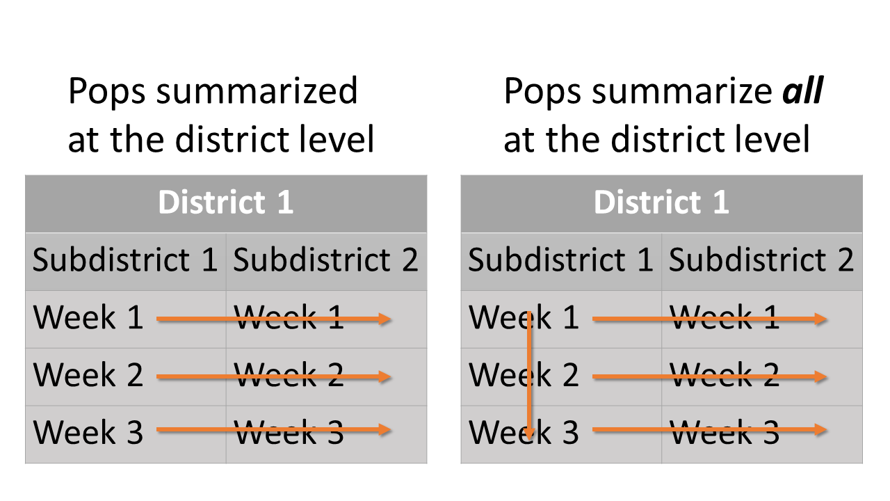
pop_summ and pop_summ_all at the district level: Summary scheme of population proportions at the district level. Oragne arrows show how different starta are summed.

For the age-by-stock composition at the district level, estimates of age class proportions are summarized for each reporting group within each district.

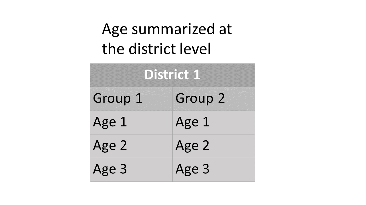
age_summ at the district level: Summary scheme of age-by-stock composition at the district level.

For the stock proportions at the subdistrict level, estimates of each statistical week are summarized for each subdistrict and each district. There is also a summary that summed up all estimated proportions of statistical weeks within each subdistrict for each district.

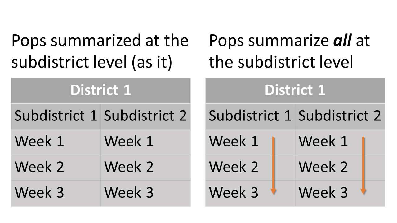
pop_summ and pop_summ_all at the subdistrict level: Summary scheme of population proportions at the subdistrict level. Oragne arrows show how different starta are summed.

For the age-by-stock composition at the subdistrict level, estimates of age class proportions are summarized for each reporting group within each subdistrict.

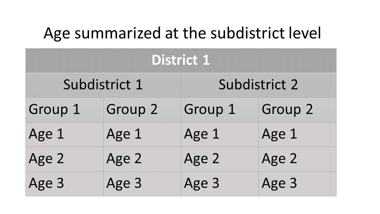
age_summ at the subdistrict level: Summary scheme of age-by-stock composition at the subdistrict level.

The summarized MAGMA output is organized as list items. The items with _summ are the summary table with posterior means, median, CrI’s and convergence diagnostics (Gelman-Rubin and effective size). At the district level, age_summ item provides summaries of age-by-stock composition within a district. pop_summ_all and pop_summ provide summaries of reporting group proportions for a district and summing across statistical weeks within a district, respectively. At the subdistrict level, age_summ item provides summaries of age-by-stock composition within each subdistrict. pop_summ_all and pop_summ provide summaries of reporting group proportions for each subdistrict and for each statistical week within a subdistrict, respectively.

An example of the summary table:

magma_summ$age_summ
#> $D1_Koyukuk
#> # A tibble: 7 × 10
#>   group  age       mean    median       sd     ci.05     ci.95    p0    GR n_eff
#>   <chr>  <fct>    <dbl>     <dbl>    <dbl>     <dbl>     <dbl> <dbl> <dbl> <dbl>
#> 1 Koyuk… 13    2.81e- 2 1.06e-  2 4.13e- 2 9.84e-  5 1.07e-  1  0.08 0.987  50  
#> 2 Koyuk… 21    2.53e- 2 1.32e-  2 3.51e- 2 1.41e-  4 1.04e-  1  0.06 1.21   50  
#> 3 Koyuk… 22    6.53e- 2 5.40e-  2 4.25e- 2 1.38e-  2 1.39e-  1  0    0.992  29.0
#> 4 Koyuk… 23    5.20e- 1 5.19e-  1 1.33e- 1 3.18e-  1 7.23e-  1  0    1.00   72.2
#> 5 Koyuk… 31    3.40e- 1 3.37e-  1 1.25e- 1 1.42e-  1 5.25e-  1  0    0.980 159. 
#> 6 Koyuk… 32    2.16e- 2 1.66e-  2 2.06e- 2 7.24e-  4 6.11e-  2  0.06 0.993  50  
#> 7 Koyuk… other 1.58e-65 6.68e-308 1.12e-64 6.68e-308 1.12e-130  1    0.981   0  
#> 
#> $D1_Tanana
#> # A tibble: 7 × 10
#>   group  age        mean    median        sd     ci.05     ci.95    p0    GR
#>   <chr>  <fct>     <dbl>     <dbl>     <dbl>     <dbl>     <dbl> <dbl> <dbl>
#> 1 Tanana 13    3.63e-  2 2.92e-  2 2.66e-  2 1.04e-  2 8.64e-  2  0    0.999
#> 2 Tanana 21    1.70e-  1 1.72e-  1 5.40e-  2 9.10e-  2 2.52e-  1  0    0.985
#> 3 Tanana 22    3.77e-  1 3.82e-  1 8.42e-  2 2.20e-  1 4.95e-  1  0    1.07 
#> 4 Tanana 23    3.91e-  1 3.77e-  1 9.25e-  2 2.61e-  1 5.42e-  1  0    1.04 
#> 5 Tanana 31    1.15e-  2 6.82e-  3 1.28e-  2 2.63e-  4 3.61e-  2  0.02 1.14 
#> 6 Tanana 32    1.38e-  2 8.95e-  3 1.67e-  2 6.12e-  4 5.05e-  2  0.02 1.01 
#> 7 Tanana other 2.62e-101 6.68e-308 1.85e-100 6.68e-308 9.47e-184  1    0.982
#> # ℹ 1 more variable: n_eff <dbl>
#> 
#> $D1_UpperUS
#> # A tibble: 7 × 10
#>   group   age       mean    median      sd     ci.05     ci.95    p0    GR n_eff
#>   <chr>   <fct>    <dbl>     <dbl>   <dbl>     <dbl>     <dbl> <dbl> <dbl> <dbl>
#> 1 UpperUS 13    0.0261   1.60e-  2 0.0394  8.40e-  4 7.76e-  2  0.04 0.998  50  
#> 2 UpperUS 21    0.0288   2.09e-  2 0.0291  8.62e-  4 8.30e-  2  0    0.984  50  
#> 3 UpperUS 22    0.324    3.15e-  1 0.0972  1.90e-  1 4.96e-  1  0    1.03   83.5
#> 4 UpperUS 23    0.178    1.81e-  1 0.0678  7.17e-  2 2.71e-  1  0    1.01   50.5
#> 5 UpperUS 31    0.0277   1.69e-  2 0.0345  1.44e-  3 8.86e-  2  0    1.12   50  
#> 6 UpperUS 32    0.415    4.11e-  1 0.0990  2.71e-  1 5.75e-  1  0    1.13   41.5
#> 7 UpperUS other 0.000202 6.68e-308 0.00142 6.68e-308 4.23e-134  0.98 1.22   25  
#> 
#> $D1_Canada
#> # A tibble: 7 × 10
#>   group  age         mean    median      sd     ci.05    ci.95    p0    GR n_eff
#>   <chr>  <fct>      <dbl>     <dbl>   <dbl>     <dbl>    <dbl> <dbl> <dbl> <dbl>
#> 1 Canada 13       5.50e-2 4.85e-  2 2.72e-2 1.89e-  2 9.97e- 2     0 1.24     50
#> 2 Canada 21       1.17e-1 1.16e-  1 4.02e-2 6.10e-  2 1.86e- 1     0 1.02     50
#> 3 Canada 22       3.69e-1 3.73e-  1 5.45e-2 2.81e-  1 4.49e- 1     0 0.984    50
#> 4 Canada 23       3.61e-1 3.58e-  1 4.94e-2 3.02e-  1 4.42e- 1     0 1.18     50
#> 5 Canada 31       4.71e-2 4.30e-  2 2.02e-2 1.91e-  2 7.73e- 2     0 1.00     50
#> 6 Canada 32       5.03e-2 4.46e-  2 2.62e-2 1.91e-  2 1.05e- 1     0 1.01     50
#> 7 Canada other    7.05e-7 6.68e-308 4.98e-6 6.68e-308 1.81e-44     1 0.982    25

$N_{eff}$ (or n_eff in the summary table) represents an estimate of independent sample size in the posterior sample. A large $N_{eff}$ is considered better than a small $N_{eff}$. Some says you would need at least blah blah number to properly estimate the credible intervals, but there is no “official” number to go by. My experience tells me to look at $N_{eff}$ together with other diagnostics. Sometimes you may see GR (Gelman-Rubin statistic, or $\hat R$) passes the test but $N_{eff}$ is small. You may want to investigate the trace plot for that particular output. Also, when the simulation iterations are small, the results for $N_{eff}$ can get wacky.

The items with “_prop” are the posterior samples/simulations (i.e., trace history) for age or population proportions in a data frame. The data frame contains output from all MCMC chains stacked together. In this example, I run two chains with 50 iterations, burn-ins of 25, and no thinning. Because I chose to keep the burn-ins, the results are 50 rows of output in each chain. Stacking the two chains we end up with 100 rows of posterior samples.

magma_summ$age_prop
#> $D1_Koyukuk
#> # A tibble: 100 × 9
#>      itr chain     other     `13`    `21`    `22`  `23`  `31`      `32`
#>    <dbl> <chr>     <dbl>    <dbl>   <dbl>   <dbl> <dbl> <dbl>     <dbl>
#>  1     1 ch1   6.68e-308 0.000118 0.0887  0.0750  0.424 0.382 0.0301   
#>  2     2 ch1   6.68e-308 0.0354   0.128   0.0426  0.505 0.289 0.000389 
#>  3     3 ch1   6.68e-308 0.0455   0.0482  0.105   0.624 0.141 0.0355   
#>  4     4 ch1   6.68e-308 0.0161   0.00362 0.00991 0.778 0.160 0.0322   
#>  5     5 ch1   6.68e-308 0.00844  0.0292  0.0234  0.490 0.449 0.000123 
#>  6     6 ch1   6.68e-308 0.00120  0.0261  0.0512  0.762 0.152 0.00674  
#>  7     7 ch1   6.68e-308 0.00861  0.00136 0.0424  0.521 0.426 0.0000256
#>  8     8 ch1   6.68e-308 0.00198  0.0358  0.135   0.624 0.203 0.0000974
#>  9     9 ch1   9.41e-179 0.190    0.00594 0.0595  0.487 0.253 0.00494  
#> 10    10 ch1   6.68e-308 0.00261  0.00844 0.103   0.458 0.429 0.000293 
#> # ℹ 90 more rows
#> 
#> $D1_Tanana
#> # A tibble: 100 × 9
#>      itr chain     other   `13`   `21`  `22`  `23`   `31`    `32`
#>    <dbl> <chr>     <dbl>  <dbl>  <dbl> <dbl> <dbl>  <dbl>   <dbl>
#>  1     1 ch1   6.68e-308 0.0567 0.165  0.291 0.363 0.0482 0.0752 
#>  2     2 ch1   6.68e-308 0.0209 0.145  0.271 0.473 0.0751 0.0151 
#>  3     3 ch1   6.68e-308 0.0130 0.202  0.366 0.317 0.0584 0.0442 
#>  4     4 ch1   6.68e-308 0.0452 0.261  0.288 0.348 0.0307 0.0271 
#>  5     5 ch1   6.68e-308 0.0585 0.229  0.304 0.390 0.0157 0.00287
#>  6     6 ch1   6.68e-308 0.0608 0.194  0.277 0.369 0.0964 0.00253
#>  7     7 ch1   6.68e-308 0.100  0.186  0.227 0.410 0.0367 0.0396 
#>  8     8 ch1   6.68e-308 0.0108 0.252  0.281 0.350 0.0918 0.0141 
#>  9     9 ch1   6.68e-308 0.0159 0.200  0.309 0.311 0.163  0.00188
#> 10    10 ch1   6.68e-308 0.0188 0.0904 0.270 0.587 0.0195 0.0143 
#> # ℹ 90 more rows
#> 
#> $D1_UpperUS
#> # A tibble: 100 × 9
#>      itr chain     other     `13`    `21`  `22`  `23`    `31`  `32`
#>    <dbl> <chr>     <dbl>    <dbl>   <dbl> <dbl> <dbl>   <dbl> <dbl>
#>  1     1 ch1   6.68e-308 0.0119   0.0804  0.146 0.216 0.0139  0.531
#>  2     2 ch1   6.68e-308 0.000790 0.0285  0.345 0.185 0.0409  0.400
#>  3     3 ch1   6.68e-308 0.0770   0.00702 0.333 0.125 0.00733 0.451
#>  4     4 ch1   6.68e-308 0.0392   0.0676  0.164 0.184 0.0803  0.464
#>  5     5 ch1   6.68e-308 0.0233   0.0458  0.198 0.261 0.0266  0.445
#>  6     6 ch1   6.68e-308 0.0140   0.0339  0.225 0.113 0.0403  0.573
#>  7     7 ch1   6.68e-308 0.0158   0.0466  0.342 0.129 0.0354  0.430
#>  8     8 ch1   6.68e-308 0.0161   0.0473  0.514 0.117 0.00139 0.305
#>  9     9 ch1   6.68e-308 0.0130   0.00378 0.412 0.177 0.0122  0.382
#> 10    10 ch1   6.68e-308 0.00234  0.0165  0.266 0.220 0.0151  0.481
#> # ℹ 90 more rows
#> 
#> $D1_Canada
#> # A tibble: 100 × 9
#>      itr chain     other   `13`   `21`  `22`  `23`   `31`   `32`
#>    <dbl> <chr>     <dbl>  <dbl>  <dbl> <dbl> <dbl>  <dbl>  <dbl>
#>  1     1 ch1   6.68e-308 0.119  0.109  0.342 0.255 0.0303 0.144 
#>  2     2 ch1   6.68e-308 0.0455 0.0893 0.481 0.304 0.0279 0.0521
#>  3     3 ch1   6.68e-308 0.107  0.0943 0.345 0.366 0.0364 0.0519
#>  4     4 ch1   9.77e- 66 0.0733 0.0692 0.186 0.614 0.0284 0.0301
#>  5     5 ch1   6.68e-308 0.0630 0.0716 0.354 0.433 0.0321 0.0463
#>  6     6 ch1   6.68e-308 0.0852 0.146  0.274 0.395 0.0498 0.0506
#>  7     7 ch1   6.68e-308 0.0279 0.138  0.382 0.358 0.0245 0.0689
#>  8     8 ch1   6.68e-308 0.0453 0.0763 0.436 0.354 0.0224 0.0666
#>  9     9 ch1   1.91e-202 0.0581 0.0962 0.468 0.317 0.0378 0.0232
#> 10    10 ch1   3.73e-152 0.0293 0.209  0.302 0.418 0.0220 0.0200
#> # ℹ 90 more rows

Trace histories can be included as a part of the summary output (default), or be saved as Fst files in a specified location. If one decided to save the trace histories as Fst, they will not be included in the summary. To save the trace histories, use the arghument save_trace to specify a location. A folder for the saved files will be automatically created. Each file is labelled based on the type, statistical district/subdistrict/week, and/or reporting group. For example, ap_d2Alaska.fst is the trace history for age proportions of district 2 for the Alaska reporting group. p_d1s2w5.fst is the trace history for group proportions of district 1, subdistrict 2, and week 5.

Trace Plot

The posterior samples trace can be used to make trace plots with your own code or with function magmatize_tr_plot(). If using magmatize_tr_plot(), you need to specify the amount of burn-ins and thinning you had when you ran the model. If you forget, you can find them in your raw magma output (e.g., magma_out$specs). magmatize_tr_plot() outputs one data frame (e.g. sampling period) at a time. The burn-in portion of the output is shaded in red.

magmatize_tr_plot(magma_summ$age_prop$D1_Koyukuk, nburn = 25)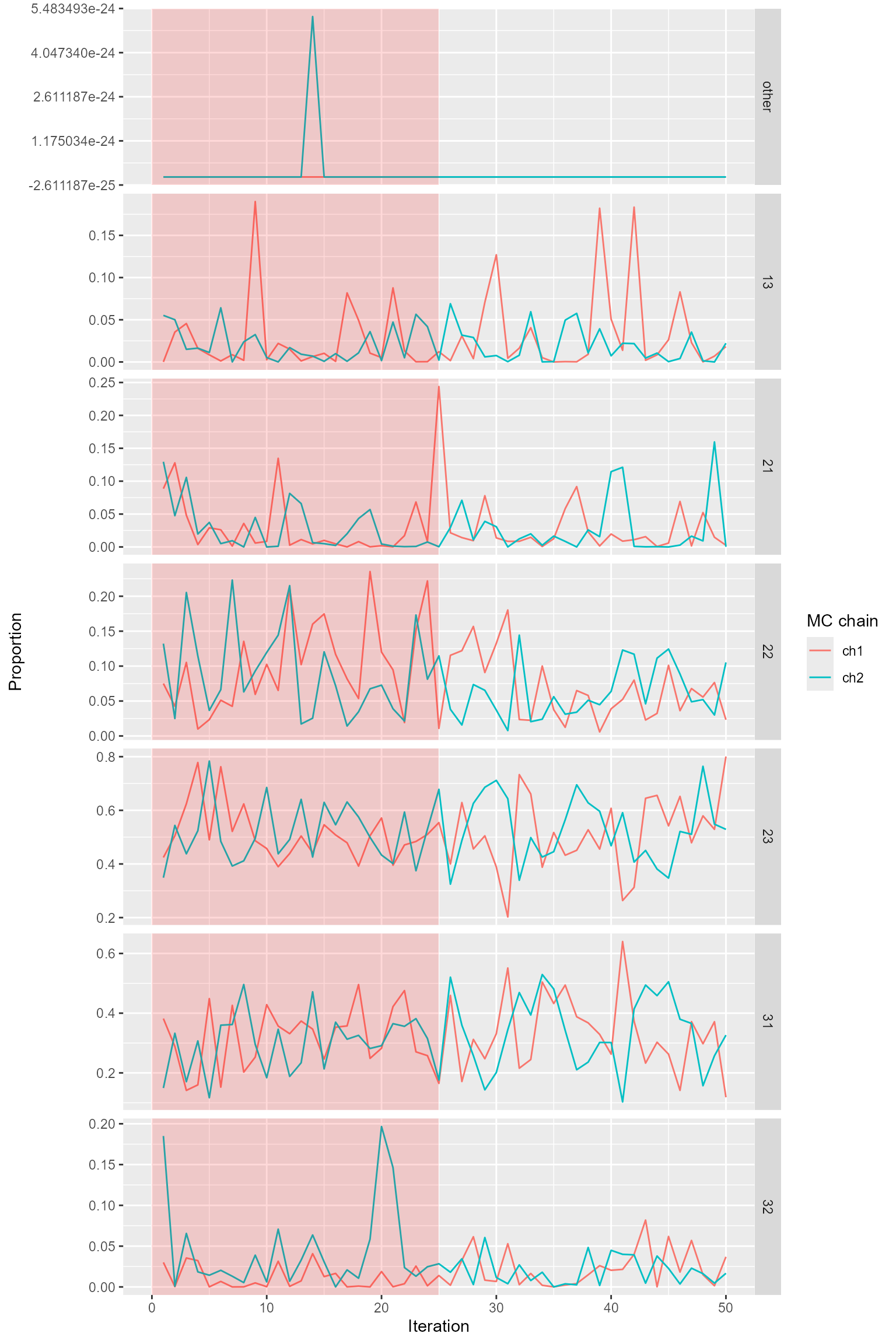

Trace plots for age composition.

Note that one can read in the saved trace histories to make trace plots. For example, trace history for age proportions of the Koyukuk reporting group can be plotted using magmatize_tr_plot(fst::read_fst(paste0(wd, "/trace_district/ap_d1Koyukuk.fst")), nburn = 25).

Individual (group membership) assignment

magmatize_indiv() summarizes the posterior means of group membership for each individual in the metadata. The probability output can be organized in populations or combined into reporting groups (for single districts only).

magma_indiv <- magmatize_indiv(ma_out = freak_out, ma_dat = yomamafat, out_repunit = TRUE)
#> Combining populations using reporting groups of district 1.

magma_indiv
#> # A tibble: 149 × 5
#>    indiv           Koyukuk Tanana UpperUS Canada
#>  * <chr>             <dbl>  <dbl>   <dbl>  <dbl>
#>  1 FAKE_KBEAV97_22    0      0       1      0   
#>  2 FAKE_KBEAV97_31    0      0       1      0   
#>  3 FAKE_KBEAV97_46    0      0       1      0   
#>  4 FAKE_KBEAV97_60    0      0       1      0   
#>  5 FAKE_KBEAV97_64    0      0       1      0   
#>  6 FAKE_KBEAV97_73    0      0       1      0   
#>  7 FAKE_KBEAV97_81    0      0       1      0   
#>  8 FAKE_KCHAN02_2     0.01   0.05    0.94   0   
#>  9 FAKE_KCHAN04_1     0      0       0.91   0.09
#> 10 FAKE_KCHAN04_16    0      0       1      0   
#> # ℹ 139 more rows

The probabilities of group memberships of each individual are based on genotype if available. Otherwise, the posteriors are based on priors or known identities, which provide no additional useful information on the group memberships. The first column of the group membership probability summary provides the unique id of each individual in the data set, which allows users to filter individuals by name.

Background and Methods

We will first introduce Pella-Masuda model in this section because it is the backbone of MAGMA. Later in the section, we will discuss how MAGMA is developed by extending the Pella-Masuda model.

Pella-Masuda Model

For a population comprised of multiple distinct groups, genetic stock identification (GSI) is used to estimate the group membership of each individual based on its genetic make-up (i.e., allele frequencies). The GSI model also estimates the overall group proportions based on the number of individuals assigned to each group. In the fishery context, genetic data of the individuals is called the mixture because it consists of multi-locus allele frequencies of individual fish collected from a mixed-stock fishery. $\mathbf x$ denotes the mixture. In this document, a bold-font letter represents a number set, or a collection of distinct elements. For example, $\mathbf x$ is a set that contains individual $x$ elements. And $x_{m,l,j}$ is the count of allele $j$ in locus $l$ for individual fish $m$, where $m \in \{1,2,...,M\}$, $l \in \{1,2,...,L\}$, and $j \in \{1,2,...,J_l\}$ depends on locus $l$.

Genetic data of the populations is called the baseline because it consists allele frequencies of various reference populations collected at their spawning locations. Researchers select sampling locations to best represent demographic production and genetic diversity of populations in an area. $\mathbf y$ denotes the baseline sample. $y_{k,l,j}$ is the count of allele $j$ in locus $l$ for a sample of size $n_{k,l}$ collected from baseline population $k$, where $k \in \{1,2,...,K\}$.

For both mixture and baseline, it is assumed that allele counts in each locus follow a multinomial distribution³. Using a made-up example, in a baseline, there are two alleles in locus 1 for population 2. Counts for the two alleles are $y_{1,2,1}, y_{1,2,2}$, and they follow a multinomial distribution with parameters $q_{1,2,1}, q_{1,2,2}$ and size $n_{2,1}$. Note that $q_{1,2,1}, q_{1,2,2}$ are the relative frequencies of the two alleles in locus 1 for population 2. In a Bayesian framework, we need to specify prior distributions for parameters; therefore, we place a Dirichlet⁴ prior distribution on $q_{1,2,1}, q_{1,2,2}$ with hyperparameters⁵ $\beta_{1,1}, \beta_{1,2}$, where $\beta_{1,1} = \beta_{1,2} = 1/2$ based on the number of alleles for locus 1.

$\mathbf q$ represents $q_{1,2,1}$ and $q_{1,2,2}$, together with allele frequencies of other loci and other populations. As you can see, $\mathbf q$ and $\mathbf y$ have the same dimension because each relative frequency corresponds to an allele count. In the model, allele frequencies of baseline populations, $\mathbf q$, determine population proportions. And population proportions is used to determine the identities of individual fish. Individual identities are then tallied and summarized to update baseline allele frequencies. $\mathbf y$ can be expressed as follows:

$\mathbf y_k \sim Mult(\mathbf n_k, \mathbf q_k)$

Prior distribution for $\mathbf q$:

$\mathbf q_k \sim Dirich(\mathbf \beta)$,

where $\mathbf \beta = 1/J_l$ is a commonly used prior for $\mathbf q$.

As mentioned, for mixture, allele counts in each locus of individual fish follows a multinomial distributions. Distribution of allele counts is related to the allele frequencies of the baseline population which the individual came from. However, the identity of the individual fish is unknown so it needs to be estimated. Here we let $\mathbf z_m$ represent the population identify for the $m$^th mixture individual. $\mathbf z_m$ is composed of 0’s and an 1 with a length $K$ (e.g. number of baseline populations). $z_{m,k} = 1$ if individual $m$ belongs to population $k$, and $z_{m,k} = 0$ otherwise. In a made-up example, $\mathbf z_{100} = \{0, 0, 1, 0, 0\}$ means that there are only five populations, and individual fish #100 comes from population 3.

We place a multinomial distribution on $z_{m,1}, z_{m,2}, ..., z_{m,K}$ with size 1 and probabilities equal to population proportions $p_1, p_2, ..., p_K$. We specify a Dirichlet prior distribution on $p_1, p_2, ..., p_K$ with hyperparameters $\alpha_1, \alpha_2, ..., \alpha_K$, where $\alpha_1 = \alpha_2 = ... = \alpha_K = 1/K$. We express $\mathbf z$ as follows:

$\mathbf z_m \sim Mult(\mathbf 1, \mathbf p)$

A commonly used prior for $\mathbf p$:

$\mathbf p \sim Dirich(\mathbf \alpha)$,

where $\mathbf \alpha = 1/K$.

As mentioned, for mixture sample, allele counts in each locus of individual fish follows a multinomial distributions. The parameters are allele frequencies of the corresponding baseline population with size the numbers of ploidy for each respective locus. Remember that population identity $z_{m,k} = 1$ if individual $m$ belongs to population $k$, and $z_{m,k} = 0$ otherwise. When multiplying population identities, $z_{m,1}, z_{m,2}, ..., z_{m,K}$, and allele frequencies of baseline populations, $\mathbf q_1, \mathbf q_2, ..., \mathbf q_K$, only allele frequencies of baseline population which individual $m$ belong to would remain while the rest goes to zero. $\mathbf x$ is expressed below.

$\mathbf x_m \sim Mult(\mathbf{ploidy}, \mathbf z_m \circ \mathbf q)$,

where $\mathbf{ploidy} = ploidy_1, ploidy_2, ..., ploidy_L$ denotes ploidy for each locus. We use $\circ$ to denote the element-wise product.

Moran and Anderson (2018) implement a genetic mixture analysis as a R package, rubias. Their program has been widely used by researchers around the world, including here at the GCL. rubias utilizes a model structure called the conditional GSI model, that is modified from the Pella-Masuda model. The main difference between the two models is that, in the conditional model, $\mathbf q$ is integrated out of the distribution of mixture sample, $\mathbf x_m$. That is, baseline allele frequencies are not being updated in the model. The result of that, $\mathbf x_m$ takes a form of a compound Dirichlet-multinomial distribution (Johnson at el., 1997):

$\mathbf x_m \sim CDM(\mathbf{ploidy}, \mathbf z_m \circ \mathbf v)$,

where $\mathbf v$ is $\mathbf \beta + \mathbf y$. We are not going to attempt proving the theory behind the conditional GSI model in this document (details can be found in Moran and Anderson, 2018). But since $\mathbf q$ has been integrated out of $\mathbf x_m$, the process for estimating parameters is simpler and more streamlined. We implemented a modified version of the conditional GSI in the updated edition of MAGMA.

Mark and Age Inclusion

MAGMA is basically Pella-Masuda model with extension to include otolith marks and aged individual fish. In Pella-Masuda model, each fish belongs to a wild population $k$, where $k \in \{1,2,...,K\}$. And their identity is estimated based on genotype. In the extended scenario, hatchery populations are added to the mixture and can be identified by their otolith markings. The identities of hatchery fish can be traced back completely to the origin $k$, where $k \in \{K+1, K+2, ..., K+H\}$.

With the addition of otolith marking, the entire mixture sample of size $M$ is now comprised of three components: 1) the number of wild fish that are genotyped $M^{(1)}$; 2) the number of wild fish that are not genotyped $M^{(2)}$; and 3) the number of otolith-marked fish $M^{(3)}$. Note that $M = M^{(1)} + M^{(2)} + M^{(3)}$.

Population identities are also partitioned into three components. $\mathbf z$ is now $\mathbf z^{(1)}$, $\mathbf z^{(2)}$, and $\mathbf z^{(3)}$, each corresponding to the respective sample-component. Compartmentalized $\mathbf z^{(i)}_m$, where $i \in \{1,2,3\}$, still follow a multinomial distribution with size 1 and parameter $\mathbf p$ as described previously. However, with the addition of hatchery populations, $\mathbf z^{(i)}_m$ and parameters $\mathbf p$ are now of length $K+H$. $p_1, p_2, ..., p_{K+H}$ have a Dirichlet distribution with hyperparameters $\alpha_1, \alpha_2, ..., \alpha_{K+H} = 1/(K+H)$. We express $\mathbf z^{(i)}$ and prior for $\mathbf p$ as follows:

$\mathbf z^{(i)}_m \sim Mult(\mathbf 1, \mathbf p)$

$\mathbf p \sim Dirich(\mathbf \alpha)$,

where $\mathbf \alpha = 1/(K+H)$

Allele counts are only available from individual fish that are genotyped; hence, genetic information is now compartmentalized to component 1 of the mixture sample:

$\mathbf x^{(1)}_m \sim Mult(\mathbf{ploidy}, \mathbf z^{(1)}_m \cdot \mathbf q)$

It is similar for the conditional GSI model:

$\mathbf x^{(1)}_m \sim CDM(\mathbf{ploidy}, \mathbf z^{(1)}_m \cdot \mathbf v)$

No genetic baseline samples are required for the hatchery populations so that the genetic baseline $y$ is unchanged from the Pella-Masuda model; however, no age-class baseline is available for any population. As described earlier, some fish in the mixture sample are aged and some are not. However, in this document we will pretend that all fish are aged so that the notation would be less headache-inducing. The fundamental concept would still be the same when not all fish were aged, only with more complicated notations.

Age class is identified as $c$, where $c \in \{1,2,...,C\}$. $\mathbf a$ denotes the age identities of mixture fish. Let $\mathbf a_m$ represent the age identify for the $m$^th mixture individual. $\mathbf a_m$ are also partitioned into three subsets, $\mathbf a^{(1)}$, $\mathbf a^{(2)}$, and $\mathbf a^{(3)}$, according to the sample-components. However, it is not necessary to compartmentalize $\mathbf a_m$ for the most part in the model. Age identity and population identity have a similar structure, and $\mathbf a_m$ is also composed of 0’s and an 1 but with a length $C$. $a_{m,c}$ is the age identity for the $m$^th mixture individual in the $c$^th age class, where $a_{m,c} = 1$ if individual $m$ has age class $c$, and $a_{m,c} = 0$ otherwise. For example, if there were three age classes and fish #6 was age 3, then $\mathbf a_6 = \{0, 0, 1\}$.

We place a multinomial distribution on $a_{m,1}, a_{m,2}, ..., a_{m,C}$ with size 1 and probabilities equal to age-class frequencies $\mathbf z_m \cdot \mathbf \pi$, where $\mathbf \pi$ denotes age-class frequencies within each population 1 through $K+H$. You can picture $\mathbf \pi$ as a matrix with $K+H$ populations of rows and $C$ age classes of columns. Therefore, when multiplying population identities, $z_{m,1}, z_{m,2}, ..., z_{m,K}$, and age-class frequencies, $\mathbf \pi_{1,\{1,2,...,C\}}, \mathbf \pi_{2,\{1,2,...,C\}}, ..., \mathbf \pi_{K+H,\{1,2,...,C\}}$, only age-class frequencies within the population which individual $m$ belong to would remain while the rest goes to zero.

We specify a Dirichlet prior on $\pi_{k,1}, \pi_{k,2}, ..., \pi_{k,C}$ with hyperparameters $\gamma_1, \gamma_2, ..., \gamma_C = 1/C$. We express $\mathbf a$ and prior for $\mathbf \pi$ as follows:

$\mathbf a_m \sim Mult(\mathbf 1, \mathbf z_m \cdot \mathbf \pi)$

$\mathbf \pi \sim Dirich(\mathbf \gamma)$,

where $\mathbf \gamma = 1/C$

Estimation of MAGMA parameters requires deriving the conditional distributions for $\mathbf p, \mathbf q, \mathbf z^{(1)}, \mathbf z^{(2)}, \mathbf\pi|\mathbf x, \mathbf y, \mathbf z^{(3)}, \mathbf a, \mathbf\alpha, \mathbf\beta, \mathbf\gamma$. In the next section, we will introduce the concepts and an algorithm to sample the posterior distribution.

MAGMA DAG: A simplified directed acyclic graph of MAGMA model. Ovals represent variables in the model. Shaded boxes represent observed variables. Diamond shapes represent the prior distributions. The large rectangles represent replication over individuals and/or loci. See main text for full explanation of the model.

Gibbs Sampler

Gibbs sampler is a type of Markov chain Monte Carlo (MCMC) methods that sequentially sample parameter values from a Markov chain. With enough sampling, the Markov chain will eventually converge to the joint posterior distribution of the parameters. The most appealing quality of Gibbs sampler is its reduction of a multivariate problem (such as Pella-Masuda and MAGMA models) to a series of more manageable lower-dimensional problems. A full description of Gibbs sampler and MCMC methods is beyond the scope of this document; however, further information can be found in numerous resources devoting to Bayesian data analysis (see Carlin & Louis, 2009; Robert & Casella, 2010; Gelman et al., 2014)

To illustrate, suppose we would like to determine the joint posterior distribution of interest, $p(\mathbf \theta|\mathbf y)$, where $\mathbf \theta = \{\theta_1, \theta_2,..., \theta_K\}$. Most likely the multivariate $p(\mathbf \theta|\mathbf y)$ would be too complicated to sample from. However, if we can figure out how to break up the joint posterior distribution into individual full conditional distributions⁶, each parameter in $\mathbf \theta$ can be sampled one by one sequentially using a Gibbs sampler algorithm. The process begins with an arbitrary set of starting values $\theta^{(0)}_2, \theta^{(0)}_3,..., \theta^{(0)}_K$ and proceeds as follows:

For $t = 1,2,...,T$, repeat

1. Draw $\theta^{(t)}_1$ from $p(\theta_1|\theta^{(t-1)}_2, \theta^{(t-1)}_3,..., \theta^{(t-1)}_k, \mathbf y)$

2. Draw $\theta^{(t)}_2$ from $p(\theta_2|\theta^{(t)}_1, \theta^{(t-1)}_3,..., \theta^{(t-1)}_k, \mathbf y)$

   ⋮

11. Draw $\theta^{(t)}_k$ from $p(\theta_k|\theta^{(t)}_1, \theta^{(t)}_2,..., \theta^{(t)}_{k-1}, \mathbf y)$

This would work best if the full conditionals are some known distributions that we can easily sample from (although it’s not required). In our case with MAGMA model, we rely on two main concepts, the Bayes theorem and conjugacy, to do the trick. Briefly, for estimating parameters $\mathbf\theta$ from data $\mathbf D$, according to Bayes Rule, $p(\mathbf\theta|\mathbf D) = \displaystyle \frac{p(\mathbf D|\mathbf\theta)p(\mathbf\theta)}{p(\mathbf D)}$. $p(\mathbf\theta|\mathbf D)$ is the joint posterior distribution for parameters $\mathbf\theta$, $p(\mathbf D|\mathbf\theta)$ is the likelihood of observing the data given the parameters, $p(\mathbf\theta)$ is the prior distribution of the parameters, and $p(\mathbf D)$ is the constant marginal distribution of the data. $p(\mathbf D)$ is often mathematically difficult to obtain; however, because $p(\mathbf D)$ is a constant number, we can ignore it by reducing the posterior distribution to $p(\mathbf\theta|\mathbf D) \propto p(\mathbf D|\mathbf\theta)p(\mathbf\theta)$.

So, how does Bayes Rule help us estimating parameters in MAGMA model? First, the joint posterior distribution has to be split up into smaller pieces. That is, we separate the joint posterior into likelihood of the data and priors for the parameters:

$p(\mathbf p, \mathbf q, \mathbf z^{(1)}, \mathbf z^{(2)}, \mathbf\pi|\mathbf x, \mathbf y, \mathbf a, \mathbf z^{(3)}, \mathbf\alpha, \mathbf\beta, \mathbf\gamma)$

$\propto p(\mathbf x|\mathbf z^{(1)}, \mathbf q) p(\mathbf y|\mathbf q) p(\mathbf a|\mathbf z,\mathbf\pi) p(\mathbf z^{(3)}|\mathbf p) \cdot p(\mathbf p|\mathbf\alpha) p(\mathbf q|\mathbf\beta) p(\mathbf z^{(1)}|\mathbf p) p(\mathbf z^{(2)}|\mathbf p) p(\mathbf \pi|\mathbf\gamma)$

$= p(\mathbf x|\mathbf z^{(1)}, \mathbf q) p(\mathbf y|\mathbf q) p(\mathbf a|\mathbf z,\mathbf\pi) \cdot p(\mathbf p|\mathbf\alpha) p(\mathbf q|\mathbf\beta) p(\mathbf z|\mathbf p) p(\mathbf \pi|\mathbf\gamma)$

With some re-arrangements and hand-waving, we arrive at the conditional distributions for $\mathbf q$, $\mathbf p$, and $\mathbf\pi$:

$p(\mathbf x|\mathbf z^{(1)}, \mathbf q) p(\mathbf y|\mathbf q) p(\mathbf a|\mathbf z,\mathbf\pi) \cdot p(\mathbf p|\mathbf\alpha) p(\mathbf q|\mathbf\beta) p(\mathbf z|\mathbf p) p(\mathbf \pi|\mathbf\gamma)$

$= p(\mathbf x|\mathbf z^{(1)}, \mathbf q) p(\mathbf y|\mathbf q) p(\mathbf q|\mathbf\beta) \cdot p(\mathbf z|\mathbf p) p(\mathbf p|\mathbf\alpha) \cdot p(\mathbf a|\mathbf z,\mathbf\pi) p(\mathbf \pi|\mathbf\gamma)$

$\propto p(\mathbf x,\mathbf y,\mathbf z^{(1)}|\mathbf q) p(\mathbf q|\mathbf\beta) \cdot p(\mathbf z|\mathbf p) p(\mathbf p|\mathbf\alpha) \cdot p(\mathbf a,\mathbf z|\mathbf\pi) p(\mathbf \pi|\mathbf\gamma)$

$\propto p(\mathbf q|\mathbf x,\mathbf y,\mathbf z^{(1)},\mathbf\beta) \cdot p(\mathbf p|\mathbf z,\mathbf\alpha) \cdot p(\mathbf \pi|\mathbf a,\mathbf z,\mathbf\gamma)$

Next, we take advantage of a mathematical property called conjugacy to help us determine the full conditional distributions. Based on this property, the posterior distribution follows the same parametric form as the prior distribution when prior is a conjugate family for the likelihood. For example, if the likelihood of data is binomial distribution and the prior of parameter is beta distribution, then the posterior is also beta distribution because beta is a conjugate family for binomial. There are many conjugate families, and Dirichlet and multinomial are another example.

Utilizing conjugacy property, we will determine each of the conditional distributions for $\mathbf q$, $\mathbf p$, and $\mathbf\pi$.

Conditional distribution p(q|x, y, z⁽¹⁾, $\beta$)

We determine that $p(\mathbf q|\mathbf x,\mathbf y,\mathbf z^{(1)},\mathbf\beta)$ is Dirichlet-distributed because Dirichlet prior $p(\mathbf q|\mathbf\beta)$ is a conjugate family for the multinomial likelihoods $p(\mathbf x|\mathbf z^{(1)}, \mathbf q)$ and $p(\mathbf y|\mathbf q)$. To determine the exact parameterization for the posterior distribution, we need to derive the prior and likelihoods first.

Likelihood $p(\mathbf x|\mathbf z^{(1)}, \mathbf q)$ can be derived in two steps. The first step we conditioned the likelihood on $\mathbf z^{(1)}$ so that

$p(\mathbf x|\mathbf z^{(1)}, \mathbf q) \propto \displaystyle \prod^{M^{(1)}}_{m=1} \prod^{K}_{k=1} [f(\mathbf x_m|\mathbf q_k)]^{z^{(1)}_{m,k}}$,

where $f(\mathbf x_m|\mathbf q_k)$ is the relative frequency of multi-locus genotype for individual $m$ in population $k$. In the next step, we derive $f(\mathbf x_m|\mathbf q_k)$:

$f(\mathbf x_m|\mathbf q_k) \propto \displaystyle \prod^{L}_{l=1} \prod^{J_l}_{j=1} q^{x_{m,l,j}}_{k,l,j}$

Then we combine the two,

$p(\mathbf x|\mathbf z^{(1)}, \mathbf q) \propto \displaystyle \prod^{M^{(1)}}_{m=1} \prod^{K}_{k=1} [f(\mathbf x_m|\mathbf q_k)]^{z^{(1)}_{m,k}}$

$\propto \displaystyle \prod^{M^{(1)}}_{m=1} \prod^{K}_{k=1} [\displaystyle \prod^{L}_{l=1} \prod^{J_l}_{j=1} q^{x_{m,l,j} \cdot z^{(1)}_{m,k}}_{k,l,j}]$

$\propto \displaystyle \prod^{K}_{k=1} \prod^{L}_{l=1} \prod^{J_l}_{j=1} q^{\sum^{M^{(1)}}_{m=1} (x_{m,l,j} \cdot z^{(1)}_{m,k})}_{k,l,j}$

Deriving likelihood $p(\mathbf y|\mathbf q)$ is more straightforward. It is the product of relative frequency of multi-locus genotype for each population:

$p(\mathbf y|\mathbf q) \propto \displaystyle \prod^{K}_{k=1} \prod^{L}_{l=1} \prod^{J_l}_{j=1} q^{y_{k,l,j}}_{k,l,j}$

And $p(q|\mathbf\beta)$ is Dirichlet prior distribution. Its probability density has a kernel⁷ of $\mathbf q^{\mathbf \beta - 1}$. We can express the likelihood as

$p(\mathbf q|\mathbf\beta) \propto \displaystyle \prod^{K}_{k=1} \prod^{L}_{l=1} \prod^{J_l}_{j=1} q^{\beta_{l,j} - 1}_{k,l,j}$.

Put all the likelihoods together,

$p(\mathbf q|\mathbf x,\mathbf y,\mathbf z^{(1)},\mathbf\beta) \propto p(\mathbf x|\mathbf z^{(1)}, \mathbf q) p(\mathbf y|\mathbf q) p(\mathbf q|\mathbf\beta)$

$\propto \displaystyle \prod^{K}_{k=1} \prod^{L}_{l=1} \prod^{J_l}_{j=1} q^{\sum^{M^{(1)}}_{m=1} (x_{m,l,j} \cdot z^{(1)}_{m,k})}_{k,l,j} \cdot \displaystyle \prod^{K}_{k=1} \prod^{L}_{l=1} \prod^{J_l}_{j=1} q^{y_{k,l,j}}_{k,l,j} \cdot \displaystyle \prod^{K}_{k=1} \prod^{L}_{l=1} \prod^{J_l}_{j=1} q^{\beta_{l,j} - 1}_{k,l,j}$

$= \displaystyle \prod^{K}_{k=1} \prod^{L}_{l=1} \prod^{J_l}_{j=1} q^{\sum^{M^{(1)}}_{m=1} (x_{m,l,j} \cdot z^{(1)}_{m,k}) + y_{k,l,j} + \beta_{l,j} - 1}_{k,l,j}$

It is elementary for anybody to recognize that $\displaystyle \prod^{K}_{k=1} \prod^{L}_{l=1} \prod^{J_l}_{j=1} q^{\sum^{M^{(1)}}_{m=1} (x_{m,l,j} \cdot z^{(1)}_{m,k}) + y_{k,l,j} + \beta_{l,j} - 1}_{k,l,j}$ is the kernel for Dirichlet distribution. Hence,

$\mathbf q_{k,l}|\mathbf x,\mathbf y,\mathbf z^{(1)},\mathbf\beta \sim Dirich(\displaystyle \sum^{M^{(1)}}_{m=1} x_{m,l,j} z^{(1)}_{m,k} + y_{k,l,j} + \beta_{l,j})$

Conditional distribution p(p|z, $\alpha$)

Using the same logic as previously, $p(\mathbf p|\mathbf z,\mathbf\alpha)$ is also Dirichlet-distributed due to a Dirichlet prior $p(\mathbf p|\mathbf\alpha)$ and a multinomial likelihood $p(\mathbf z|\mathbf p)$.

$p(\mathbf p|\mathbf z,\mathbf\alpha) \propto p(\mathbf z|\mathbf p) p(\mathbf p|\mathbf\alpha)$

$\propto \displaystyle \prod^{M}_{m=1} \prod^{K+H}_{k=1} p^{z_{m,k}}_k \cdot \prod^{K+H}_{k=1} p^{\alpha_k - 1}_k$

$\propto \displaystyle \prod^{K+H}_{k=1} p^{\sum^M_{m=1}z_{m,k} + \alpha_k - 1}_k$

Once again, we recognize it as the kernel for Dirichlet distribution:

$\mathbf p|\mathbf z,\mathbf\alpha \sim Dirich(\displaystyle \sum^M_{m=1}z_{m,k} + \alpha_k)$

Conditional distribution p($\pi$|a, z, $\gamma$)

Lastly, $p(\mathbf \pi|\mathbf a,\mathbf z,\mathbf\gamma)$ is also Dirichlet-distributed due to a Dirichlet prior $p(\mathbf \pi|\mathbf\gamma)$ and a multinomial likelihood $p(\mathbf a|\mathbf z,\mathbf\pi)$.

$p(\mathbf \pi|\mathbf a,\mathbf z,\mathbf\gamma) \propto p(\mathbf a|\mathbf z,\mathbf\pi) p(\mathbf \pi|\mathbf\gamma)$

$\propto \displaystyle \prod^{M}_{m=1}\prod^{K+H}_{k=1}[h(\mathbf a_m|\mathbf\pi_k)]^{z_{m,k}} \cdot \prod^{K+H}_{k=1}\prod^{C}_{c=1}\pi^{\gamma_c - 1}_{k,c}$,

where likelihood $h(\mathbf a_m|\mathbf\pi_k) \propto \displaystyle \prod^C_{c=1}\pi^{a_{m,k}}_{k,c}$ is the product of relative frequency of age class for individual $m$ in population $k$. Plugging in $h(\mathbf a_m|\mathbf\pi_k)$,

$\displaystyle \prod^{M}_{m=1}\prod^{K+H}_{k=1}[h(\mathbf a_m|\mathbf\pi_k)]^{z_{m,k}} \cdot \prod^{K+H}_{k=1}\prod^{C}_{c=1}\pi^{\gamma_c - 1}_{k,c}$

$= \displaystyle \prod^{M}_{m=1}\prod^{K+H}_{k=1}[\displaystyle \prod^C_{c=1}\pi^{a_{m,k}z_{m,k}}_{k,c}] \cdot \prod^{K+H}_{k=1}\prod^{C}_{c=1}\pi^{\gamma_c - 1}_{k,c}$

$= \displaystyle \prod^{K+H}_{k=1}\displaystyle \prod^C_{c=1}\pi^{\sum^M_{m=1}a_{m,k}z_{m,k}}_{k,c} \cdot \prod^{K+H}_{k=1}\prod^{C}_{c=1}\pi^{\gamma_c - 1}_{k,c}$

$= \displaystyle \prod^{K+H}_{k=1}\displaystyle \prod^C_{c=1}\pi^{\sum^M_{m=1}a_{m,k}z_{m,k}+ \gamma_c - 1}_{k,c}$

And we recognize it as the kernel for Dirichlet distribution:

$\mathbf \pi_k|\mathbf a, \mathbf z, \mathbf\gamma \sim Dirich(\displaystyle \sum^M_{m=1}a_{m,k}z_{m,k} + \gamma_c)$

Algorithm

There is one more distribution to figure out before we can start our Gibbs sampler routine (and you thought we’re all set, lol). We would need to know how to sample $\mathbf z^{(1,2)}_m|\mathbf p, \mathbf q, \mathbf x^{(1,2)}_m, \mathbf\pi, \mathbf a^{(1,2)}_m$, the population identity for individual fish $m$ (in components 1 and 2) given the population proportions, genotype, and age. If the probability of fish $m$ belong to population $k$ is $p_k$, and the likelihood of observing relative frequency of genotype and age class for fish $m$ in population $k$ is $f(\mathbf x^{(1,2)}_m|\mathbf q_k) \cdot h(\mathbf a^{(1,2)}_m|\mathbf\pi_k)$, then the probability of fish $m$ belong to population $k$ given the population proportions genotype, and age is $\displaystyle \frac{p_k \cdot f(\mathbf x^{(1,2)}_m|\mathbf q_k) \cdot h(\mathbf a^{(1,2)}_m|\mathbf\pi_k)}{\sum^K_{k'=1}p_{k'} \cdot f(\mathbf x^{(1,2)}_m|\mathbf q_{k'}) \cdot h(\mathbf a^{(1,2)}_m|\mathbf\pi_{k'})}$. The denominator should sum to one, so we only need to calculate the numerator. $\mathbf z^{(1,2)}_m|\mathbf p, \mathbf q, \mathbf x^{(1,2)}_m, \mathbf\pi, \mathbf a^{(1,2)}_m$ has the following distribution:

$\mathbf z^{(1,2)}_m|\mathbf p, \mathbf q, \mathbf x^{(1,2)}_m, \mathbf\pi, \mathbf a^{(1,2)}_m \sim Mult(1, \mathbf{p'}_m)$,

where $p'_{m,k} = p_k \cdot f(\mathbf x^{(1,2)}_m|\mathbf q_k) \cdot h(\mathbf a^{(1,2)}_m|\mathbf\pi_k)$. We draw the initial values for $\mathbf q_k$ and $\mathbf \pi_k$ based on their prior distributions.

Once we figured out all the pieces in the Gibbs sampler, we may begin the process with starting values for $\mathbf p^{(0)}$, $\mathbf q^{(0)}$, and $\mathbf \pi^{(0)}$. If not all fish were aged, $\mathbf a^{(1,2)(0)}_m$ at the initial step would contain all 0’s for those individuals without an assigned age. Which is not a problem because age class will be determined in the subsequent steps. We proceed as follows:

For $t = 1,2,...,T$, repeat

1. Determine the population membership of mixture individuals, ${{\mathbf z}^{(1,2)}_m}^{(t)}|\mathbf p^{(t-1)}, \mathbf q^{(t-1)}, \mathbf x^{(1,2)}_m, \mathbf\pi^{(t-1)}, {{\mathbf a}^{(1,2)}_m}^{(t-1)} \sim Mult(1, \mathbf {p'}_m)$.

2. If not all individuals were aged, determine memberships of age classes for those with unknown age, $\mathbf a^{(t)}_m|\mathbf z^{(t)}_m, \mathbf \pi^{(t-1)} \sim Mult(1, \mathbf z^{(t)}_m \mathbf\pi^{(t-1)})$.

3. Draw updated values for $\mathbf q^{(t)}$, $\mathbf p^{(t)}$, and $\mathbf\pi^{(t)}$ from $p(\mathbf q|\mathbf x,\mathbf y,{{\mathbf z}^{(1)}}^{(t)},\mathbf\beta)$, $p(\mathbf p|\mathbf z^{(t)},\mathbf \alpha)$, and $p(\mathbf \pi|\mathbf a^{(t)},\mathbf z^{(t)},\mathbf \gamma)$ respectively.

$T$ should be large enough to ensure the sampler chain converges to the posterior distribution of the parameters. Usually it takes thousands of iterations. That completes the Gibbs sampler process. Whew.

Implementing the conditional GSI model only requires a slight modification from the above algorithm. Basically, $f(\mathbf x^{(1,2)}_m|\mathbf q_k)$ would only need to be derived once in the beginning of the process, and $\mathbf q$ would no longer need to be updated in step 3. Everything else would stay the same.

we eventually realized that a purely conditional GSI algorithm would not work for MAGMA because the baseline allele frequencies needed to be updated so that the age frequencies would be updated as well. Instead, we adapted an algorithm that is the hybrid of conditional and fully Bayesian GSI. Mainly, we would run the model in the conditional GSI algorithm with the fully Bayesian algorithm at every 10^th iteration.

References

Carlin, B. and T. Louis. 2009. Bayesian Methods for Data Analysis, 3rd Edition. CRC Press. New York.

Gelman, A., J. Carlin, H. Stern, D. Dunson, A. Vehtari and D. Rubin. Bayesian Data Analysis, 3rd Edition. CRC Press. New York.

Johnson, N.L., Kotz, S., and Balakrishnan, N. 1997. Discrete multivariate distributions. Wiley & Sons, New York.

Moran, B.M. and E.C. Anderson. 2018. Bayesian inference from the conditional genetic stock identification model. Canadian Journal of Fisheries and Aquatic Sciences. 76(4):551-560. https://doi.org/10.1139/cjfas-2018-0016

Pella, J. and M. Masuda. 2001. Bayesian methods for analysis of stock mixtures from genetic characters. Fish. Bull. 99:151–167.

Robert, C. and G. Casella. 2010. Introducing Monte Carlo Methods with R. Springer. New York.