*Ms.GSI* in the multistage of genetic stock identification madness

library(Ms.GSI)
# devtools::load_all()

Overview

This document contains the background information for a integrated multistage genetic stock identification (GSI) model in two parts. The first part the describes how to use package Ms.GSI to conduct a GSI analysis. The steps include formatting input data, running the integrated multistage GSI model, and summarizing results. The second part details the technical background of integrated multistage GSI model and its mathematical theory. There is a separate article describe the general background of the integrated multistage framework (add link to integrated multistage paper).

How to use Ms.GSI

Ms.GSI follows the work flow: format input data, run integrated multistage model, and summarize results/convergence diagnostics.

Input data

There are few pieces of information needed for input data set:

broad-scale baseline
regional baseline
mixture sample
broad-scale population information
regional population information

There are pre-loaded example data sets available in Ms.GSI. We will look at them one at a time. Note that the example data sets are simulated using existing baseline archived by the Alaska Department of Fish & Game Gene Conservation Lab (GCL). The fabricated data set does not represent the true population proportions in real fisheries. In this example, we made up a scenario similar to the Bering Sea groundfish fisheries where Chinook salmon harvested as bycatch originated from a wide range of geographic areas. Within the bycatch sample, we were interested in the proportion contribution from the lower, middle and upper Yukon River reporting groups (see map below). We used a coast-wide data set for Chinook salmon (Templin et al. 2011; Templin baseline hereafter) as the broad-scale baseline to separate Yukon River fish from other non-Yukon stocks in our data set during the first stage of the analysis. However, genetic markers in the Templin baseline were unable to clearly distinguish between lower Yukon River and other coastal western Alaska populations, so we used a second baseline with additional genetic markers that were specifically designed to differentiate Yukon River Chinook salmon populations (Lee et al. 2021; Yukon River baseline hereafter) as the regional fine-scale baseline for the second stage.

It is important to note that in the original grouping of the Templin baseline, Lower Yukon was a part of Coastal Western Alaska reporting group. We isolated Lower Yukon from the rest of the Coastal Western Alaska, but the accuracy of the proportion estimates would likely diminish because of the breakup of Coastal Western Alaska reporting group. We do not recommend using a genetic baseline beyond its original design. And researchers should be aware of the capability of their genetic baselines before utilizing them in the integrated multistage model. In our example, it would be ideal to keep the Coastal Western Alaska group intact in the broad-scale baseline, and break up the group into Lower Yukon and others using a fine-scale regional baseline. However, at the time of writing, such regional baseline with adequate resolution was still in development.

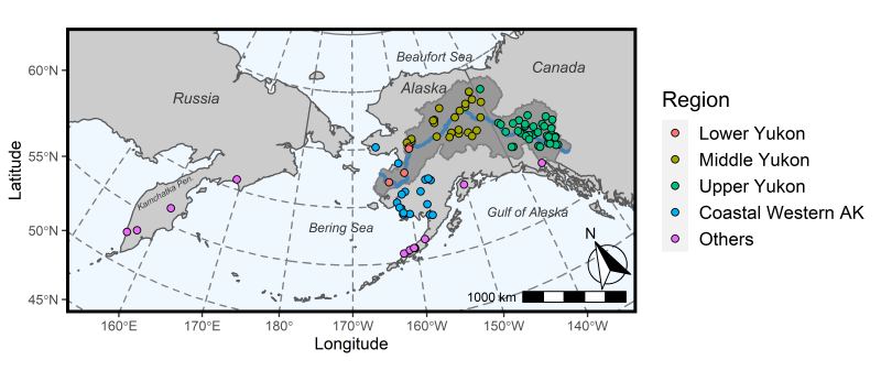
Collection locations and color-coded reporting groups of Chinook salmon represented in the Yukon River example. Shaded area represents the Yukon River region.

We assembled a mixture sample containing 150 individuals from collection sites across Yukon River, coastal western Alaskan, Alaska Peninsula, Gulf of Alaska, and Kamchatka Peninsula (Russia). The collections were grouped into five reporting groups: Lower Yukon, Middle Yukon, Upper Yukon, Coastal Western Alaska (Coastal West Alaska), and Others.

Mixture

First we will take a look at the baseline and mixture samples. Ms.GSI accepts the genotype information in two format: 1) GCL format or 2) package rubias format. The example data sets are in rubias format and naming convention, but procedures for GCL format are the same¹.


print(dplyr::as_tibble(mix))
#> # A tibble: 150 × 358
#>    sample_type repunit collection indiv   `GTH2B-550` `GTH2B-550.1` NOD1  NOD1.1
#>    <chr>       <lgl>   <chr>      <chr>   <chr>       <chr>         <chr> <chr> 
#>  1 mixture     NA      Bering Sea fish_1  C           G             C     C     
#>  2 mixture     NA      Bering Sea fish_2  C           C             C     G     
#>  3 mixture     NA      Bering Sea fish_3  C           C             C     G     
#>  4 mixture     NA      Bering Sea fish_4  C           C             C     C     
#>  5 mixture     NA      Bering Sea fish_5  C           G             C     G     
#>  6 mixture     NA      Bering Sea fish_6  C           C             C     G     
#>  7 mixture     NA      Bering Sea fish_7  C           C             NA    NA    
#>  8 mixture     NA      Bering Sea fish_8  C           G             NA    NA    
#>  9 mixture     NA      Bering Sea fish_9  C           G             C     G     
#> 10 mixture     NA      Bering Sea fish_10 C           G             NA    NA    
#> # ℹ 140 more rows
#> # ℹ 350 more variables: `Ots_100884-287` <chr>, `Ots_100884-287.1` <chr>,
#> #   `Ots_101554-407` <chr>, `Ots_101554-407.1` <chr>, `Ots_102414-395` <chr>,
#> #   `Ots_102414-395.1` <chr>, `Ots_102867-609` <chr>, `Ots_102867-609.1` <chr>,
#> #   `Ots_103041-52` <chr>, `Ots_103041-52.1` <chr>, `Ots_103122-180` <chr>,
#> #   `Ots_103122-180.1` <chr>, `Ots_104048-194` <chr>, `Ots_104048-194.1` <chr>,
#> #   `Ots_104063-132` <chr>, `Ots_104063-132.1` <chr>, `Ots_104415-88` <chr>, …

Columns 5 to 358 contain genotype information for loci in BOTH broad-scale and regional baselines. You do not have to specify the loci for each baseline (you can if you want to double check, more on that later). Ms.GSI matches the loci between mixture and baselines as long as the locus names are consistent.

If you have fish with known-origin, you can specify their identities by adding a column called known_collection in the mixture data set. The entry for known-origin should match the collection name in the broad-scale baseline. Fish with unknown-origin should have a NA entry.

Broad-scale baseline

Next, we will take a look at the broad-scale (Templin) baseline example provided in Ms.GSI. There are originally 45 loci in the Templin baseline, but we reduced the marker set to 28 loci due to limitation on the data size (and other technical reasons). However, for demonstration purpose, this data set will suffice.


print(dplyr::as_tibble(base_templin))
#> # A tibble: 29,363 × 60
#>    sample_type repunit collection indiv   `GTH2B-550` `GTH2B-550.1` NOD1  NOD1.1
#>    <chr>       <chr>   <chr>      <chr>   <chr>       <chr>         <chr> <chr> 
#>  1 reference   Russia  KBIST98L   KBIST9… C           C             C     G     
#>  2 reference   Russia  KBIST98L   KBIST9… C           G             C     G     
#>  3 reference   Russia  KBIST98L   KBIST9… C           G             C     G     
#>  4 reference   Russia  KBIST98L   KBIST9… C           C             G     G     
#>  5 reference   Russia  KBIST98L   KBIST9… C           G             G     G     
#>  6 reference   Russia  KBIST98L   KBIST9… C           C             C     C     
#>  7 reference   Russia  KBIST98L   KBIST9… C           G             C     G     
#>  8 reference   Russia  KBIST98L   KBIST9… C           C             C     G     
#>  9 reference   Russia  KBIST98L   KBIST9… C           G             C     G     
#> 10 reference   Russia  KBIST98L   KBIST9… C           C             G     G     
#> # ℹ 29,353 more rows
#> # ℹ 52 more variables: `Ots_2KER-137` <chr>, `Ots_2KER-137.1` <chr>,
#> #   `Ots_AsnRS-72` <chr>, `Ots_AsnRS-72.1` <chr>, Ots_ETIF1A <chr>,
#> #   Ots_ETIF1A.1 <chr>, `Ots_GPH-318` <chr>, `Ots_GPH-318.1` <chr>,
#> #   `Ots_GST-207` <chr>, `Ots_GST-207.1` <chr>, `Ots_hnRNPL-533` <chr>,
#> #   `Ots_hnRNPL-533.1` <chr>, `Ots_HSP90B-100` <chr>, `Ots_HSP90B-100.1` <chr>,
#> #   `Ots_IGF1-91` <chr>, `Ots_IGF1-91.1` <chr>, `Ots_IK1-328` <chr>, …

Regional baseline

The regional baseline (Yukon) is in the same format. There are originally 380 loci in the Yukon River Chinook baseline, but we reduced the numbers to 177 in this demonstration.


print(dplyr::as_tibble(base_yukon))
#> # A tibble: 5,435 × 358
#>    sample_type repunit   collection indiv `GTH2B-550` `GTH2B-550.1` NOD1  NOD1.1
#>    <chr>       <chr>     <chr>      <chr> <chr>       <chr>         <chr> <chr> 
#>  1 reference   Lower Yu… KANDR02.K… KAND… G           G             C     C     
#>  2 reference   Lower Yu… KANDR02.K… KAND… C           G             C     C     
#>  3 reference   Lower Yu… KANDR02.K… KAND… G           G             C     C     
#>  4 reference   Lower Yu… KANDR02.K… KAND… G           G             C     G     
#>  5 reference   Lower Yu… KANDR02.K… KAND… C           G             C     C     
#>  6 reference   Lower Yu… KANDR02.K… KAND… C           C             C     C     
#>  7 reference   Lower Yu… KANDR02.K… KAND… C           G             G     G     
#>  8 reference   Lower Yu… KANDR02.K… KAND… C           C             G     G     
#>  9 reference   Lower Yu… KANDR02.K… KAND… C           C             G     G     
#> 10 reference   Lower Yu… KANDR02.K… KAND… C           G             C     G     
#> # ℹ 5,425 more rows
#> # ℹ 350 more variables: `Ots_100884-287` <chr>, `Ots_100884-287.1` <chr>,
#> #   `Ots_101554-407` <chr>, `Ots_101554-407.1` <chr>, `Ots_102414-395` <chr>,
#> #   `Ots_102414-395.1` <chr>, `Ots_102867-609` <chr>, `Ots_102867-609.1` <chr>,
#> #   `Ots_103041-52` <chr>, `Ots_103041-52.1` <chr>, `Ots_103122-180` <chr>,
#> #   `Ots_103122-180.1` <chr>, `Ots_104048-194` <chr>, `Ots_104048-194.1` <chr>,
#> #   `Ots_104063-132` <chr>, `Ots_104063-132.1` <chr>, `Ots_104415-88` <chr>, …

Population information

Another piece of information needed is the population details for each baseline. You need to include three columns in the population information table. Column collection contains the names for each population in the baseline. Column reunit specifies the reporting group each population belongs to. Column grpvec specifies the identification number for each reporting group. Below shows the first ten rows of population information for the Templin (broad-scale) baseline.


print(dplyr::as_tibble(templin_pops211))
#> # A tibble: 211 × 3
#>    collection       repunit             grpvec
#>    <chr>            <chr>                <dbl>
#>  1 KBIST98L         Russia                   1
#>  2 KBOLS02.KBOLS98E Russia                   1
#>  3 KKAMC97.KKAMC98L Russia                   1
#>  4 KPAKH02          Russia                   1
#>  5 KPILG05.KPILG06  Coastal West Alaska      2
#>  6 KUNAL05          Coastal West Alaska      2
#>  7 KGOLS05.KGOLS06  Coastal West Alaska      2
#>  8 KANDR02.KANDR03  Lower Yukon              3
#>  9 KANVI02          Lower Yukon              3
#> 10 KGISA01          Lower Yukon              3
#> # ℹ 201 more rows

If you have hatchery populations in your mixture sample, you can tell Ms.GSI either a collection belongs to natural or hatchery-origin by adding an origin column in the population information table. In the origin column, you identify each collection with "wild" or "hatchery". If you don’t care to separate natural and hatchery origins, you can lump them in one collection. In this case, you don’t need to add an origin column. Also, this option to identify hatchery fish is only available in the broad-scale baseline, so don’t add an origin column in the population table for regional baseline.

Population information table for the Yukon (regional) baseline is in the same format, but not necessarily in the same order.


print(dplyr::as_tibble(yukon_pops50))
#> # A tibble: 50 × 3
#>    collection                          grpvec repunit     
#>    <chr>                                <dbl> <chr>       
#>  1 KANDR02.KANDR03                          1 Lower Yukon 
#>  2 KANVI03.KANVI07                          1 Lower Yukon 
#>  3 KNUL12SF                                 1 Lower Yukon 
#>  4 KNUL12NF                                 1 Lower Yukon 
#>  5 KGISA01                                  1 Lower Yukon 
#>  6 KKATE02.KKATE12                          1 Lower Yukon 
#>  7 KHENS01                                  2 Middle Yukon
#>  8 KHENS07.KHENS15                          2 Middle Yukon
#>  9 KSFKOY03                                 2 Middle Yukon
#> 10 KMFKOY10.KMFKOY11.KMFKOY12.KMFKOY13      2 Middle Yukon
#> # ℹ 40 more rows

Once you have the data files ready (I recommend saving them as .Rdata or .Rds files), you can use prep_msgsi_data() function to convert them into input data set for model run. You’ll also need to identify “groups of interest” in parameter sub-group. In this example, groups of interests are Lower Yukon, Middle Yukon and Upper Yukon reporting groups. Their identify numbers are 3, 4, and 5 in the broad-scale baseline. There’s an option to save the input data at a designated directory by identifying the location in parameter file_path.

prep_msgsi_data() function matches the loci between mixture and baselines. But if you want to make sure that you didn’t miss any locus in your baselines or mixture, you can manually provide loci names (in string vector) for each baseline by inputting them in loci1 and loci2. In this example we don’t manually provide lists of loci because we trust that mixture and baselines all have the correct loci.


msgsi_dat <-
  prep_msgsi_data(mixture_data = mix,
  baseline1_data = base_templin, baseline2_data = base_yukon,
  pop1_info = templin_pops211, pop2_info = yukon_pops50, sub_group = 3:5)
#> Compiling input data, may take a minute or two...
#> Time difference of 9.539811 secs

prep_msgsi_data() formats the data files and put them in a list. It took few seconds to format the input data in this case. Bigger data sets may take longer. Here are the first few rows/items in the input data list:


lapply(msgsi_dat, head)
#> $x
#> # A tibble: 6 × 74
#>   indiv    `GTH2B-550_1` `GTH2B-550_2` NOD1_1 NOD1_2 `Ots_2KER-137_1`
#>   <chr>            <int>         <int>  <int>  <int>            <int>
#> 1 fish_1               1             1      2      0                0
#> 2 fish_10              1             1      0      0                1
#> 3 fish_100             1             1      1      1                1
#> 4 fish_101             1             1      1      1                1
#> 5 fish_102             0             2      0      2                0
#> 6 fish_103             2             0      1      1                1
#> # ℹ 68 more variables: `Ots_2KER-137_2` <int>, `Ots_2KER-137_3` <int>,
#> #   `Ots_AsnRS-72_1` <int>, `Ots_AsnRS-72_2` <int>, `Ots_AsnRS-72_3` <int>,
#> #   Ots_ETIF1A_1 <int>, Ots_ETIF1A_2 <int>, `Ots_GPH-318_1` <int>,
#> #   `Ots_GPH-318_2` <int>, `Ots_GST-207_1` <int>, `Ots_GST-207_2` <int>,
#> #   `Ots_HSP90B-100_1` <int>, `Ots_HSP90B-100_2` <int>, `Ots_IGF1-91_1` <int>,
#> #   `Ots_IGF1-91_2` <int>, `Ots_IGF1-91_3` <int>, `Ots_IK1-328_1` <int>,
#> #   `Ots_IK1-328_2` <int>, `Ots_IK1-328_3` <int>, `Ots_LEI-292_1` <int>, …
#> 
#> $x2
#> # A tibble: 6 × 355
#>   indiv    `GTH2B-550_1` `GTH2B-550_2` NOD1_1 NOD1_2 `Ots_100884-287_1`
#>   <chr>            <int>         <int>  <int>  <int>              <int>
#> 1 fish_1               1             1      2      0                  2
#> 2 fish_10              1             1      0      0                  0
#> 3 fish_100             1             1      1      1                  1
#> 4 fish_101             1             1      1      1                  2
#> 5 fish_102             2             0      0      2                  1
#> 6 fish_103             0             2      1      1                  1
#> # ℹ 349 more variables: `Ots_100884-287_2` <int>, `Ots_101554-407_1` <int>,
#> #   `Ots_101554-407_2` <int>, `Ots_102414-395_1` <int>,
#> #   `Ots_102414-395_2` <int>, `Ots_102867-609_1` <int>,
#> #   `Ots_102867-609_2` <int>, `Ots_103041-52_1` <int>, `Ots_103041-52_2` <int>,
#> #   `Ots_103122-180_1` <int>, `Ots_103122-180_2` <int>,
#> #   `Ots_104048-194_1` <int>, `Ots_104048-194_2` <int>,
#> #   `Ots_104063-132_1` <int>, `Ots_104063-132_2` <int>, …
#> 
#> $y
#> # A tibble: 6 × 76
#>   collection            repunit grpvec `GTH2B-550_1` `GTH2B-550_2` NOD1_1 NOD1_2
#>   <chr>                 <chr>    <dbl>         <int>         <int>  <int>  <int>
#> 1 CHBIG92.KIBIG93.KBIG… Northe…      9           254            82    104    228
#> 2 CHCRY92.KICRY94.KCRY… Coasta…     10           306           302    120    488
#> 3 CHDMT92.KDEER94       Coasta…     10           178           116     77    217
#> 4 CHKAN92.KIKAN93.KKAN… Coasta…      2           341           147    281    199
#> 5 CHKOG92.KIKOG93.KKOG… Coasta…      2           205            91    191    105
#> 6 CHNUU92.KINUS93       Coasta…      2            85            27     73     41
#> # ℹ 69 more variables: `Ots_2KER-137_1` <int>, `Ots_2KER-137_2` <int>,
#> #   `Ots_2KER-137_3` <int>, `Ots_AsnRS-72_1` <int>, `Ots_AsnRS-72_2` <int>,
#> #   `Ots_AsnRS-72_3` <int>, Ots_ETIF1A_1 <int>, Ots_ETIF1A_2 <int>,
#> #   `Ots_GPH-318_1` <int>, `Ots_GPH-318_2` <int>, `Ots_GST-207_1` <int>,
#> #   `Ots_GST-207_2` <int>, `Ots_HSP90B-100_1` <int>, `Ots_HSP90B-100_2` <int>,
#> #   `Ots_IGF1-91_1` <int>, `Ots_IGF1-91_2` <int>, `Ots_IGF1-91_3` <int>,
#> #   `Ots_IK1-328_1` <int>, `Ots_IK1-328_2` <int>, `Ots_IK1-328_3` <int>, …
#> 
#> $y2
#> # A tibble: 6 × 357
#>   collection            grpvec repunit `GTH2B-550_1` `GTH2B-550_2` NOD1_1 NOD1_2
#>   <chr>                  <dbl> <chr>           <int>         <int>  <int>  <int>
#> 1 CHSID92j                   3 Upper …             7           183    116     74
#> 2 K100MILECR16.K100MIL…      3 Upper …             7           103     78     34
#> 3 KANDR02.KANDR03            1 Lower …            78           230    208    100
#> 4 KANVI03.KANVI07            1 Lower …            62           164    131     79
#> 5 KBEAV97                    2 Middle…            40           148    152     38
#> 6 KBIGS87.KBIGS07            3 Upper …            30           258    231     65
#> # ℹ 350 more variables: `Ots_100884-287_1` <int>, `Ots_100884-287_2` <int>,
#> #   `Ots_101554-407_1` <int>, `Ots_101554-407_2` <int>,
#> #   `Ots_102414-395_1` <int>, `Ots_102414-395_2` <int>,
#> #   `Ots_102867-609_1` <int>, `Ots_102867-609_2` <int>,
#> #   `Ots_103041-52_1` <int>, `Ots_103041-52_2` <int>, `Ots_103122-180_1` <int>,
#> #   `Ots_103122-180_2` <int>, `Ots_104048-194_1` <int>,
#> #   `Ots_104048-194_2` <int>, `Ots_104063-132_1` <int>, …
#> 
#> $iden
#> NULL
#> 
#> $nalleles
#>    GTH2B-550         NOD1 Ots_2KER-137 Ots_AsnRS-72   Ots_ETIF1A  Ots_GPH-318 
#>            2            2            3            3            2            2 
#> 
#> $nalleles2
#>      GTH2B-550           NOD1 Ots_100884-287 Ots_101554-407 Ots_102414-395 
#>              2              2              2              2              2 
#> Ots_102867-609 
#>              2 
#> 
#> $groups
#> # A tibble: 6 × 3
#>   collection                      repunit                  grpvec
#>   <chr>                           <chr>                     <dbl>
#> 1 CHBIG92.KIBIG93.KBIGB04.KBIGB95 Northeast Gulf of Alaska      9
#> 2 CHCRY92.KICRY94.KCRYA05         Coastal Southeast Alaska     10
#> 3 CHDMT92.KDEER94                 Coastal Southeast Alaska     10
#> 4 CHKAN92.KIKAN93.KKANE05         Coastal West Alaska           2
#> 5 CHKOG92.KIKOG93.KKOGR05         Coastal West Alaska           2
#> 6 CHNUU92.KINUS93                 Coastal West Alaska           2
#> 
#> $p2_groups
#> # A tibble: 6 × 3
#>   collection                repunit      grpvec
#>   <chr>                     <chr>         <dbl>
#> 1 CHSID92j                  Upper Yukon       3
#> 2 K100MILECR16.K100MILECR15 Upper Yukon       3
#> 3 KANDR02.KANDR03           Lower Yukon       1
#> 4 KANVI03.KANVI07           Lower Yukon       1
#> 5 KBEAV97                   Middle Yukon      2
#> 6 KBIGS87.KBIGS07           Upper Yukon       3
#> 
#> $comb_groups
#> # A tibble: 6 × 3
#>   collection                      repunit                  grpvec
#>   <chr>                           <chr>                     <dbl>
#> 1 CHBIG92.KIBIG93.KBIGB04.KBIGB95 Northeast Gulf of Alaska      9
#> 2 CHCRY92.KICRY94.KCRYA05         Coastal Southeast Alaska     10
#> 3 CHDMT92.KDEER94                 Coastal Southeast Alaska     10
#> 4 CHKAN92.KIKAN93.KKANE05         Coastal West Alaska           2
#> 5 CHKOG92.KIKOG93.KKOGR05         Coastal West Alaska           2
#> 6 CHNUU92.KINUS93                 Coastal West Alaska           2
#> 
#> $sub_group
#> [1] 3 4 5
#> 
#> $group_names_t1
#> [1] "Russia"                 "Coastal West Alaska"    "Lower Yukon"           
#> [4] "Middle Yukon"           "Upper Yukon"            "North Alaska Peninsula"
#> 
#> $group_names_t2
#> [1] "Lower Yukon"  "Middle Yukon" "Upper Yukon" 
#> 
#> $wildpops
#> [1] "CHBIG92.KIBIG93.KBIGB04.KBIGB95" "CHCRY92.KICRY94.KCRYA05"        
#> [3] "CHDMT92.KDEER94"                 "CHKAN92.KIKAN93.KKANE05"        
#> [5] "CHKOG92.KIKOG93.KKOGR05"         "CHNUU92.KINUS93"                
#> 
#> $hatcheries
#> NULL

Genetic stock identification

Once your input data set is ready, you can use msgsi_mdl() to run the model. If you are used to running rubias, Ms.GSI might feel a bit slow. That is because 1) we are running two GSI models in tandem, so it takes twice as long than running a single model, and 2) Ms.GSI is written solely in R, which is not as computationally efficient as language C. So, why not code Ms.GSI in C? Because we’re not technically advanced like the folks who developed rubias package (i.e., we don’t know how to code in C++).

Because of the running time, we recommend running the integrated multistage model in conditional GSI mode (default setting). But there is an option to run the model in fully Bayesian mode if one choose to. If you run the model in fully Bayesian mode, you have the option to include numbers of adaptation run. Some people think that adaptation run encourages convergence in fully Bayesian mode. We have not test that theory but provide the option for those who want to try it.

We demonstrate the model run with one chains of 150 iterations (first 50 as warm-up runs, or burn-ins). We only run one chain in this example so it can pass CMD check while building the vignette document². In reality, you should definitely run multiple chains with more iterations. There are also options to keep the burn-ins and set random seed for reproducible results. We don’t show them in this example though (but you can always ?msgsi_mdl).


msgsi_out <- msgsi_mdl(msgsi_dat, nreps = 150, nburn = 50, thin = 1, nchains = 1)
#> Running model (and the category is... Linen Vs. Silk!)
#> Time difference of 2.26746 secs
#> April-25-2025 19:10

Summarizing results

Stock proportions

The output of model contains eight items: summ_t1, trace_t1, summ_t2, trace_t2, summ_comb, trace_comb, comb_groups, iden_t1 and idens_t2. Items with “summ” are summary for reporting group proportions and associated convergence diagnostics. If you want to see summaries for stage one and two individually, summ_t1 and summ_t2 will show you that. Most people probably want to see the combined summary, summ_comb.


msgsi_out$summ_comb
#> # A tibble: 12 × 9
#>    group                mean  median      sd    ci.05   ci.95    p0 GR     n_eff
#>    <chr>               <dbl>   <dbl>   <dbl>    <dbl>   <dbl> <dbl> <lgl>  <dbl>
#>  1 Russia            3.94e-2 3.90e-2 2.15e-2 1.24e- 2 0.0738   0    NA     25.7 
#>  2 Coastal West Ala… 1.01e-1 5.84e-2 1.05e-1 7.83e-13 0.289    0.17 NA      2.74
#>  3 North Alaska Pen… 3.14e-2 2.58e-2 2.30e-2 1.07e- 9 0.0692   0.08 NA     22.6 
#>  4 Northwest Gulf o… 2.55e-1 2.49e-1 6.97e-2 1.55e- 1 0.379    0    NA     16.6 
#>  5 Copper            3.04e-4 3.53e-6 7.76e-4 1.84e-18 0.00197  0.41 NA     54.0 
#>  6 Northeast Gulf o… 4.85e-3 1.21e-5 1.18e-2 4.06e-16 0.0298   0.36 NA      7.71
#>  7 Coastal Southeas… 2.18e-3 7.16e-6 5.48e-3 1.91e-16 0.0131   0.39 NA     25.2 
#>  8 British Columbia  5.95e-4 8.70e-7 1.51e-3 1.05e-20 0.00462  0.48 NA    100   
#>  9 WA/OR/CA          3.49e-4 9.68e-7 8.16e-4 2.41e-18 0.00234  0.45 NA     29.7 
#> 10 Lower Yukon       3.17e-1 2.99e-1 1.03e-1 1.75e- 1 0.490    0    NA      3.54
#> 11 Middle Yukon      6.67e-2 6.56e-2 2.32e-2 3.48e- 2 0.107    0    NA     62.2 
#> 12 Upper Yukon       1.82e-1 1.81e-1 2.92e-2 1.36e- 1 0.231    0    NA    100

Most column names are self explanatory, but others might need some additional descriptions. ci.05 and ci.95 are the lower and upper bounds of 90% credible interval. GR is the Gelman-Rubin statistic (a.k.a. $\hat R$ ). In this example, Gelman-Rubin statistic is not calculated because we only run one chain. n_eff is the effective size, or $N_{eff}$ . We will not discuss how to diagnose convergence in this document. Please consult Gelman et al. 2014, Gelman & Rubin 1992, Brooks & Gelman 1998 and other literature on statistical methods.

Items with “trace” are the posterior sample history, or trace history, for either stage one, two, or combined. Trace history is needed for making trace plots. And if you need to combine reporting groups proportions or combine variance, trace histories are what you need. trace_ items are tibbles with each collection as a column. There are two additional columns, itr and chain, to identify Markov chain Monte Carlo (MCMC) sampling iteration and chain.

comb_groups are provided in the output as reference for trace plot and stratified estimator. Grouping for stage one and two can also be found in the input data.


msgsi_out$trace_comb
#> # A tibble: 100 × 238
#>    CHBIG92.KIBIG93.KBIGB04.KBIGB95 CHCRY92.KICRY94.KCRYA05 CHDMT92.KDEER94
#>                              <dbl>                   <dbl>           <dbl>
#>  1                        3.23e-47               1.80e-172       6.16e- 31
#>  2                        5.80e- 7               1.61e-101       8.97e- 63
#>  3                        7.12e-40               1.31e-123       6.78e- 14
#>  4                        2.16e-15               2.42e-124       2.23e-308
#>  5                        1.38e-26               3.17e- 32       5.69e-283
#>  6                        1.66e- 3               2.23e-308       9.08e- 82
#>  7                        1.27e-67               2.23e-308       7.83e- 53
#>  8                        4.11e-41               3.03e- 48       4.36e- 22
#>  9                        1.60e-24               2.23e-308       1.69e- 62
#> 10                        1.08e-30               3.22e- 35       4.91e-198
#> # ℹ 90 more rows
#> # ℹ 235 more variables: CHKAN92.KIKAN93.KKANE05 <dbl>,
#> #   CHKOG92.KIKOG93.KKOGR05 <dbl>, CHNUU92.KINUS93 <dbl>,
#> #   CHTAH92.KTAHI04 <dbl>, CHWHI92.KWHIT98.KWHITC05 <dbl>, KALSE04 <dbl>,
#> #   KANCH06.KANCH10 <dbl>, KANDR89.KANDR04 <dbl>, KAROL05 <dbl>,
#> #   KBENJ05.KBENJ06 <dbl>, KBIGCK04 <dbl>, KBIGQU96 <dbl>,
#> #   KBIRK01.KBIRK02.KBIRK03.KBIRK97.KBIRK99 <dbl>, KBIST98L <dbl>, …

Individual assignments

The last two items in the output are the identity assignment history of each individual in the mixture sample. Each column represents an individual in the mixture, and each row records the identity assigned during each iteration in each chain. These numbers are the population identifiers in the same order as your population information files (and baseline files). Individuals are ordered in the same as the input data (i.e., mixture data).


msgsi_out$idens_t1
#> # A tibble: 100 × 150
#>       V1    V2    V3    V4    V5    V6    V7    V8    V9   V10   V11   V12   V13
#>    <int> <int> <int> <int> <int> <int> <int> <int> <int> <int> <int> <int> <int>
#>  1   116    15    11   141   141    15    97   141   116   114   141   116   141
#>  2   141    69   141   141   141    11    97   141   141    23   141   157    11
#>  3   116   116    21   141   141    23    97   141   141   114    83   157    11
#>  4    69    69    21    11   116   152    97   141    11    21    11   141    69
#>  5   141    21    21   141   116    15    97   141    97   114    11   141    11
#>  6    69   157    21    11    97    23    97   141   141   114   114   141   152
#>  7   141   157    97    11   141    11    97   141    69   114    11   114    69
#>  8   141    11    21   116   141    11    97   141   141    11   141   157    69
#>  9    69   111    25    11   114   152    97   141    11   141    69   157   141
#> 10   141    69    25   116    97   152    97   116    97    11   116   141    11
#> # ℹ 90 more rows
#> # ℹ 137 more variables: V14 <int>, V15 <int>, V16 <int>, V17 <int>, V18 <int>,
#> #   V19 <int>, V20 <int>, V21 <int>, V22 <int>, V23 <int>, V24 <int>,
#> #   V25 <int>, V26 <int>, V27 <int>, V28 <int>, V29 <int>, V30 <int>,
#> #   V31 <int>, V32 <int>, V33 <int>, V34 <int>, V35 <int>, V36 <int>,
#> #   V37 <int>, V38 <int>, V39 <int>, V40 <int>, V41 <int>, V42 <int>,
#> #   V43 <int>, V44 <int>, V45 <int>, V46 <int>, V47 <int>, V48 <int>, …

Individual identity output in this format may not be very useful for most users. So, Ms.GSI has a function indiv_assign() that summarize the reporting group assignment probabilities for each individual in the mixture.


indiv_assign(mdl_out = msgsi_out, mdl_dat = msgsi_dat)
#> # A tibble: 150 × 13
#>    ID       Russia `Coastal West Alaska` `North Alaska Peninsula`
#>  * <chr>     <dbl>                 <dbl>                    <dbl>
#>  1 fish_1     0.01                  0.25                     0   
#>  2 fish_10    0.05                  0.11                     0.06
#>  3 fish_100   0.52                  0.05                     0.02
#>  4 fish_101   0.01                  0.17                     0   
#>  5 fish_102   0                     0.18                     0.08
#>  6 fish_103   0                     0.07                     0   
#>  7 fish_104   0                     0                        0   
#>  8 fish_105   0                     0.08                     0   
#>  9 fish_106   0                     0.08                     0   
#> 10 fish_107   0.01                  0                        0.24
#> # ℹ 140 more rows
#> # ℹ 9 more variables: `Northwest Gulf of Alaska` <dbl>, Copper <dbl>,
#> #   `Northeast Gulf of Alaska` <dbl>, `Coastal Southeast Alaska` <dbl>,
#> #   `British Columbia` <dbl>, `WA/OR/CA` <dbl>, `Lower Yukon` <dbl>,
#> #   `Middle Yukon` <dbl>, `Upper Yukon` <dbl>

The summary for individual assignment has a column named ID that identifies each individual in the mixture. Not regional column shows the probability of an individual not belong to the group of interest, or, not from within region of focus. The rest of the columns are probabilities for the regional reporting groups. Probabilities in each row should sum up to one.

Trace plot

Ms.GSI has a function for you to make trace plot and examine the mixing of MCMC chains. Don’t forget to include the group information (as in groups, p2_groups, or comb_groups) for the trace history that you want to plot.


tr_plot(obj = msgsi_out$trace_comb, pop_info = msgsi_out$comb_groups)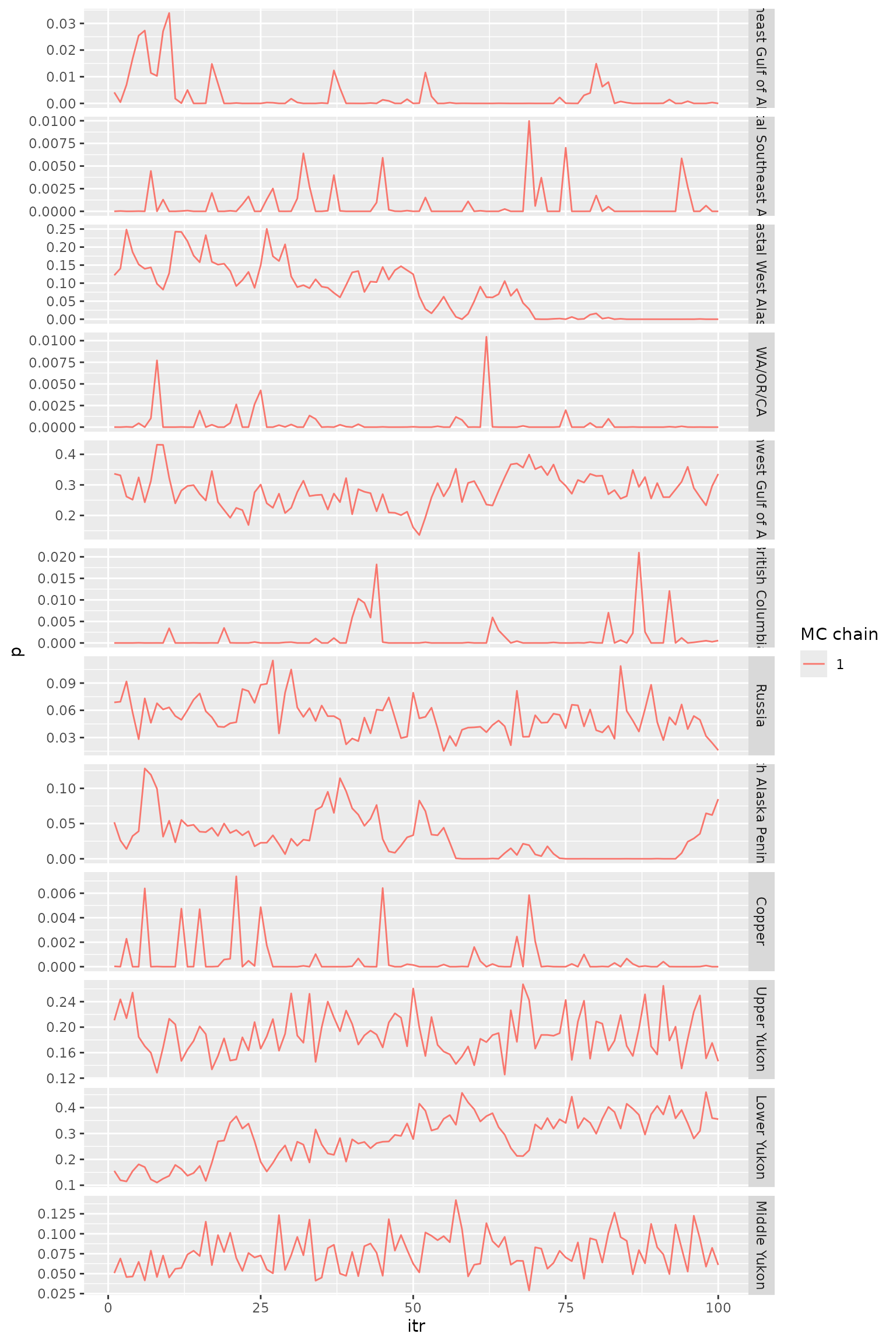

Trace plots for reporting group proportions.

Methods (math!)

Pella-Masuda Model

This integrated multistage GSI model is essentially two Bayesian GSI models stacked on top of each other; hence the name “multistage.” The Pella-Masuda model (Pella & Masuda 2001) is the Bayesian GSI model that make up each stage in the integrated multistage model. We will first describe the Pella-Masuda model before discussing the development of a integrated multistage model.

In a group of mixed populations, Pella-Masuda model assigns population identities to each individual based on its genetic make-up (e.g. genotype). Then the model estimates the overall population proportions based on the numbers of individuals assigned to each population. In the fishery context, genetic data of the individuals is called the mixture sample because it consists multi-locus genotype of individual fish collected from a mixed-stock fishery. $\mathbf x$ denotes the mixture sample. In this document, a bold-font letter represents a number set, or a collection of distinct elements. For example, $\mathbf x$ is a set that contains individual $x$ elements. And $x_{m,l,j}$ is the count of allele $j$ in locus $l$ for individual fish $m$ , where $m \in \{1,2,...,M\}$ , $l \in \{1,2,...,L\}$ , and $j \in \{1,2,...,J_l\}$ depends on locus $l$ .

Genetic data of the populations is called the baseline sample because it consists genotype compositions of various baseline populations collected at their spawning locations. Researchers select sampling locations to best represent the populations in an area. $\mathbf y$ denotes the baseline sample. $y_{k,l,j}$ is the count of allele $j$ in locus $l$ for a sample of size $n_{k,l}$ collected from baseline population $k$ , where $k \in \{1,2,...,K\}$ .

For both mixture and baseline samples, it is assumed that allele counts in each locus follow a multinomial distribution³. Using another made-up example, in a baseline sample, there are two allele types in locus 1 for population 2. Counts for the two alleles are $y_{1,2,1}, y_{1,2,2}$ , and they follow a multinomial distribution with parameters $q_{1,2,1}, q_{1,2,2}$ and size $n_{2,1}$ . Note that $q_{1,2,1}, q_{1,2,2}$ are the relative frequencies of the two alleles in locus 1 for population 2. In a Bayesian framework, we need to specify prior distributions for parameters; therefore, we place a Dirichlet⁴ prior distribution on $q_{1,2,1}, q_{1,2,2}$ with hyperparameters⁵ $\beta_{1,1}, \beta_{1,2}$ . Usually we set the priors to be equal for all loci. In this example, let $\beta_{1,1} = \beta_{1,2} = 1/2$ based on the number of alleles for locus 1.

$\mathbf q$ represents $q_{1,2,1}$ and $q_{1,2,2}$ , together with allele frequencies of other loci and other populations. As you can see, $\mathbf q$ and $\mathbf y$ have the same dimension because each relative frequency corresponds to an allele count. In the model, allele frequencies of baseline populations, $\mathbf q$ , determine population proportions. And population proportions determines the identities of individual fish. Individual identities are then tallied and summarized to update baseline allele frequencies. $\mathbf y$ can be expressed as follows:

$\mathbf y_k \sim Mult(\mathbf n_k, \mathbf q_k)$

Prior distribution for $\mathbf q$ :

$\mathbf q_k \sim Dirich(\mathbf \beta)$ ,

where $\mathbf \beta = 1/J_l$

For mixture sample, allele counts in each locus of individual fish also follows a multinomial distributions. If a fish came from a certain population, its distribution of allele counts should resemble the allele frequencies of the baseline population which it came from. However, the identity of the individual fish is unknown so it needs to be estimated. Here we let $\mathbf z_m$ represent the population identify for the $m$ ^th mixture individual. $\mathbf z_m$ is composed of 0’s and an 1 with a length $K$ (e.g. number of baseline populations). $z_{m,k} = 1$ if individual $m$ belongs to population $k$ , and $z_{m,k} = 0$ otherwise. In a made-up example, $\mathbf z_{100} = \{0, 0, 1, 0, 0\}$ means that there are five baseline populations, and individual fish #100 comes from population 3.

We place a multinomial prior on $z_{m,1}, z_{m,2}, ..., z_{m,K}$ with size 1 and probabilities equal to population proportions $p_1, p_2, ..., p_K$ . We specify a Dirichlet prior distribution on $p_1, p_2, ..., p_K$ with hyperparameters $\alpha_1, \alpha_2, ..., \alpha_K$ , where $\alpha_1 = \alpha_2 = ... = \alpha_K = 1/K$ . We usually set $\alpha$ to be equal for all reporting groups, but they can be set based on prior knowledge in population proportions. We express $\mathbf z$ as follows:

$\mathbf z_m \sim Mult(\mathbf 1, \mathbf p)$

Prior distribution for $\mathbf p$ :

$\mathbf p \sim Dirich(\mathbf \alpha)$ ,

where $\mathbf \alpha = 1/K$

As mentioned, for mixture sample, allele counts in each locus of individual fish follows a multinomial distributions. The parameters are allele frequencies of the corresponding baseline population with size the numbers of ploidy for each respective locus. Remember that population identity $z_{m,k} = 1$ if individual $m$ belongs to population $k$ , and $z_{m,k} = 0$ otherwise. When multiplying population identities, $z_{m,1}, z_{m,2}, ..., z_{m,K}$ , and allele frequencies of baseline populations, $\mathbf q_1, \mathbf q_2, ..., \mathbf q_K$ , only allele frequencies of baseline population which individual $m$ belong to would remain while the rest goes to zero. $\mathbf x$ is expressed below. $\mathbf{ploidy} = ploidy_1, ploidy_2, ..., ploidy_L$ denotes ploidy for each locus.

$\mathbf x_m \sim Mult(\mathbf{ploidy}, \mathbf z_m \cdot \mathbf q)$

Moran and Anderson (2018) implement a genetic mixture analysis as a R package, rubias. Their program has been widely used by researchers around the world, including here at the GCL. rubias utilizes a model structure called the conditional genetic stock identification model, or the conditional GSI model, that is modified from the Pella-Masuda model. The main difference between the two models is that, in the conditional model, $\mathbf q$ is integrated out of the distribution of mixture sample, $\mathbf x_m$ . That is, baseline allele frequencies are not being updated in the model. The result of that, $\mathbf x_m$ takes a form of a compound Dirichlet-multinomial distribution (Johnson at el. 1997):

$\mathbf x_m \sim CDM(\mathbf{ploidy}, \mathbf z_m \cdot \mathbf v)$ ,

where $\mathbf v$ is $\mathbf \beta + \mathbf y$ . We are not going to attempt proving the theory behind the conditional model in this document (details can be found in Moran & Anderson 2018). But since $\mathbf q$ has been integrated out of $\mathbf x_m$ , the process for estimating parameters is simpler and more streamlined. We have implemented conditional GSI in each stage of our integrated multistage model.

Extend to multistage

In a multistage setting, we refer to a baseline that covers the whole range of a mixed stock fishery as a broad-scale baseline. The broad-scale baseline typically covers a wide range of geographic areas but does not have a comprehensive collection of reference populations nor genetic markers to resolve differences between local populations within a sub-region. These smaller sub-regions of a broad-scale baseline are covered by regional baselines with higher resolutions. We generalize the conditions of the Ms.GSI model to allow multiple regional baselines to be included, although we programmed Ms.GSI to deal with only one regional baseline vs. one broad-scale baseline.

Let there be $B$ populations in the broad-scale baseline and indexed as $b = 1, 2, ..., B$ . Each of these broad-scale populations may belong to exactly 0 or 1 sub-region for which regional baselines might be available. These regional baselines have different sets of genetic markers than the broad-scale baseline and typically include additional populations that are not represented in the broad-scale baseline. Allow for there to be $R$ disjoint sub-regions indexed by $r$ , with each sub-region represented by a distinctive regional baseline. We employ a superscript $^{(r)}$ upon variables to indicate a quantity associated with regional baseline $r$ . Populations in different sub-regions cannot overlap, and each population only occurs once among the regional baselines. Let $k$ index the populations within these $R$ regional baselines and $K_r$ denotes the number of populations within regional baseline $r$ .

In the Ms.GSI framework, the two stages are connected because the regional group membership of an individual is conditional on whether the broad-scale group membership of that individual belongs to the area of that particular sub-region. The following describes the conditional relationship between the broad-scale and the regional baselines:

$\mathbf z^{(r)}_m | \mathbf z_m, \mathbf {\mathscr B}^{(r)} = \begin{cases} \mathbf z^{(r)}_m & \text{if } \sum_{b \in \mathbf{\mathscr B}^{(r)}} z_{m,b} = 1\\ \mathbf 0 & \text{otherwise} \end{cases}$ ,

where $\mathbf z_m$ and $\mathbf z^{(r)}_m$ are vectors of indicators ( $0$ or $1$ ) identifying the broad-scale and regional populations that individual $m$ belongs to. $\mathbf{\mathscr B}^{(r)}$ denotes the broad-scale populations that belong to the areas represented by the reporting groups of region $r$ , and $\mathbf 0$ is a vector of all zeros.

Ultimately, we want to estimate the fraction of individuals in the mixture that come from each of the sub-regional populations, as well as from any of the populations in the broad-scale baseline that are not associated with a regional baseline. $p^{(r)}_k$ denotes the mixture proportion of the $k$ ^th population in region $r$ , and $p_b$ denotes the mixture proportion of population $b$ in the broad-scale baseline. Thus, we endeavor to estimate the mixture proportions $p^{(r)}_k$ for each $(r, k)$ such that $r = 1, 2, ..., R$ and $k = 1, 2, ..., K_r$ along with $p_b$ , where $b \in \mathbf{\mathscr B_{*}}$ , with $\mathbf{\mathscr B_{*}}$ denoting the broad-scale populations that do not belong to any areas represented by regional baselines. Lastly, we multiply $\mathbf {p}^{(r)}$ by $\sum_{b \in \mathbf{\mathscr B}^{(r)}} p_b$ for each region $r$ , so the scaled $\mathbf{p}^{(r)}$ for all regions and $p_b$ , where $b \in \mathbf{\mathscr B_{*}}$ would sum to one.

Gibbs Sampler: where the fun go round and round

Deriving the values of parameters in each stage of the integrated multistage model requires finding the joint posterior distribution of Pella-Masuda model in each stage, $\mathbf p, \mathbf q,\mathbf z, \mathbf y, \mathbf\alpha, \mathbf\beta$ . In this section, we will introduce the concepts and algorithm to sample from this posterior distribution in a single baseline Pella-Masuda model, which then can be extend to an integrated multistage framework.

Gibbs sampler is a type of MCMC methods that sequentially sample parameter values from a Markov chain. With enough sampling, the Markov chain will eventually converge to the desire distribution of interest. The most appealing quality of Gibbs sampler is its reduction of a multivariate problem (such as Pella-Masuda model) to a series of more manageable lower-dimensional problems. A full description of Gibbs sampler and MCMC methods is beyond the scope of this document; however, further information can be found in numerous resources devoting to Bayesian data analysis (see Carlin & Louis 2009; Robert & Casella 2010; Gelman et al. 2014)

To illustrate, suppose we would like to determine the joint posterior distribution of interest, $p(\mathbf \theta|\mathbf y)$ , where $\mathbf \theta = \{\theta_1, \theta_2,..., \theta_K\}$ . Most likely the multivariate $p(\mathbf \theta|\mathbf y)$ would be too complicated to sample from. However, if we can figure out how to break up the joint posterior distribution into individual full conditional distributions, each parameter in $\mathbf \theta$ can be sampled one by one sequentially using a Gibbs sampler algorithm. The process begins with an arbitrary set of starting values $\theta^{(0)}_2, \theta^{(0)}_3,..., \theta^{(0)}_K$ and proceeds as follows:

For $t = 1,2,...,T$ , repeat

Draw $\theta^{(t)}_1$ from $p(\theta_1|\theta^{(t-1)}_2, \theta^{(t-1)}_3,..., \theta^{(t-1)}_k, \mathbf y)$
Draw $\theta^{(t)}_2$ from $p(\theta_2|\theta^{(t)}_1, \theta^{(t-1)}_3,..., \theta^{(t-1)}_k, \mathbf y)$

⋮

Draw $\theta^{(t)}_k$ from $p(\theta_k|\theta^{(t)}_1, \theta^{(t)}_2,..., \theta^{(t)}_{k-1}, \mathbf y)$

This would work best if the full conditionals are some known distributions that we can easily sample from (although it’s not required). In our case with Pella-Masuda model, we rely on two main concepts, the Bayes theorem and conjugacy, to do the trick. Briefly, for estimating parameters $\mathbf\theta$ from data $\mathbf D$ , according to Bayes Rule, $p(\mathbf\theta|\mathbf D) = \displaystyle \frac{p(\mathbf D|\mathbf\theta)p(\mathbf\theta)}{p(\mathbf D)}$ . $p(\mathbf\theta|\mathbf D)$ is the joint posterior distribution for parameters $\mathbf\theta$ , $p(\mathbf D|\mathbf\theta)$ is the likelihood of observing the data given the parameters, $p(\mathbf\theta)$ is the prior distribution of the parameters, and $p(\mathbf D)$ is the constant marginal distribution of the data. $p(\mathbf D)$ is often mathematically difficult to obtain; however, because $p(\mathbf D)$ is a constant number, we can ignore it by reducing the posterior distribution to $p(\mathbf\theta|\mathbf D) \propto p(\mathbf D|\mathbf\theta)p(\mathbf\theta)$ .

So, how does Bayes Rule help us estimating parameters in the Pella-Masuda model? First, the joint posterior distribution has to be split up into smaller pieces. That is, we separate the joint posterior into likelihood of the data and priors for the parameters:

$p(\mathbf p, \mathbf q, \mathbf z, \mathbf y, \mathbf\alpha, \mathbf\beta)$

With some re-arrangements and hand-waving, we arrive at the full conditional distributions for $\mathbf q$ and $\mathbf p$ :

$\propto p(\mathbf x,\mathbf y,\mathbf z|\mathbf q) p(\mathbf q|\mathbf\beta) \cdot p(\mathbf z|\mathbf p) p(\mathbf p|\mathbf\alpha)$

$\propto p(\mathbf q|\mathbf x,\mathbf y,\mathbf z,\mathbf\beta) \cdot p(\mathbf p|\mathbf z,\mathbf\alpha)$

Next, we take advantage of a mathematical property called conjugacy to help us determine the conditional distributions. Based on this property, the posterior distribution follows the same parametric form as the prior distribution when prior is a conjugate family for the likelihood. For example, if the likelihood of data is binomial distribution and the prior of parameter is beta distribution, then the posterior is also beta distribution because beta is a conjugate family for binomial. There are many conjugate families, and Dirichlet and multinomial are another example.

Utilizing conjugacy property, we will determine each of the full conditional distributions for $\mathbf q$ and $\mathbf p$ .

Conditional distribution p(q|x, y, z, $\beta$ )

We determine that $p(\mathbf q|\mathbf x, \mathbf y, \mathbf z, \mathbf \beta)$ is Dirichlet-distributed because Dirichlet prior $p(\mathbf q|\mathbf \beta)$ is a conjugate family for the multinomial likelihoods $p(\mathbf x|\mathbf z, \mathbf q)$ and $p(\mathbf y|\mathbf q)$ . To determine the exact parameterization for the posterior distribution, we need to derive the prior and likelihoods first.

Likelihood $p(\mathbf x|\mathbf z, \mathbf q)$ can be derived in two steps. The first step we conditioned the likelihood on $\mathbf z$ so that

$p(\mathbf x|\mathbf z, \mathbf q) \propto \displaystyle \prod^{M}_{m=1} \prod^{K}_{k=1} [f(\mathbf x_m|\mathbf q_k)]^{z_{m,k}}$ ,

where $f(\mathbf x_m|\mathbf q_k)$ is the relative frequency of multi-locus genotype for individual $m$ in population $k$ . In the next step, we derive $f(\mathbf x_m|\mathbf q_k)$ :

$f(\mathbf x_m|\mathbf q_k) \propto \displaystyle \prod^{L}_{l=1} \prod^{J_l}_{j=1} q^{x_{m,l,j}}_{k,l,j}$

Then we combine the two,

$p(\mathbf x|\mathbf z, \mathbf q) \propto \displaystyle \prod^{M}_{m=1} \prod^{K}_{k=1} [f(\mathbf x_m|\mathbf q_k)]^{z_{m,k}}$

$\propto \displaystyle \prod^{M}_{m=1} \prod^{K}_{k=1} [\displaystyle \prod^{L}_{l=1} \prod^{J_l}_{j=1} q^{x_{m,l,j} \cdot z_{m,k}}_{k,l,j}]$

$\propto \displaystyle \prod^{K}_{k=1} \prod^{L}_{l=1} \prod^{J_l}_{j=1} q^{\sum^{M}_{m=1} (x_{m,l,j} \cdot z_{m,k})}_{k,l,j}$

Deriving likelihood $p(\mathbf y|\mathbf q)$ is more straightforward. It is the product of relative frequency of multi-locus genotype for each population:

$p(\mathbf y|\mathbf q) \propto \displaystyle \prod^{K}_{k=1} \prod^{L}_{l=1} \prod^{J_l}_{j=1} q^{y_{k,l,j}}_{k,l,j}$

And $p(q|\mathbf \beta)$ is Dirichlet prior distribution. Its probability density has a kernel⁶ of $\mathbf q^{\mathbf \beta - 1}$ . We can express the likelihood as

$p(\mathbf q|\mathbf \beta) \propto \displaystyle \prod^{K}_{k=1} \prod^{L}_{l=1} \prod^{J_l}_{j=1} q^{\beta_{l,j} - 1}_{k,l,j}$ .

Put all the likelihoods together,

$p(\mathbf q|\mathbf x,\mathbf y,\mathbf z,\mathbf\beta) \propto p(\mathbf x|\mathbf z, \mathbf q) p(\mathbf y|\mathbf q) p(\mathbf q|\mathbf\beta)$

$\propto \displaystyle \prod^{K}_{k=1} \prod^{L}_{l=1} \prod^{J_l}_{j=1} q^{\sum^{M}_{m=1} (x_{m,l,j} \cdot z_{m,k})}_{k,l,j} \cdot \displaystyle \prod^{K}_{k=1} \prod^{L}_{l=1} \prod^{J_l}_{j=1} q^{y_{k,l,j}}_{k,l,j} \cdot \displaystyle \prod^{K}_{k=1} \prod^{L}_{l=1} \prod^{J_l}_{j=1} q^{\beta_{l,j} - 1}_{k,l,j}$

$= \displaystyle \prod^{K}_{k=1} \prod^{L}_{l=1} \prod^{J_l}_{j=1} q^{\sum^{M}_{m=1} (x_{m,l,j} \cdot z_{m,k}) + y_{k,l,j} + \beta_{l,j} - 1}_{k,l,j}$

It is elementary to recognize that $\displaystyle \prod^{K}_{k=1} \prod^{L}_{l=1} \prod^{J_l}_{j=1} q^{\sum^{M}_{m=1} (x_{m,l,j} \cdot z_{m,k}) + y_{k,l,j} + \beta_{l,j} - 1}_{k,l,j}$ is the kernel for Dirichlet distribution. Hence,

$\mathbf q_{k,l}|\mathbf x,\mathbf y,\mathbf z,\mathbf\beta \sim Dirich(\displaystyle \sum^{M}_{m=1} x_{m,l,j} z_{m,k} + y_{k,l,j} + \beta_{l,j})$ .

Conditional distribution p(p|z, $\alpha$ )

Using the same logic as previously, $p(\mathbf p|\mathbf z,\mathbf\alpha)$ is also Dirichlet-distributed due to a Dirichlet prior $p(\mathbf p|\mathbf\alpha)$ and a multinomial likelihood $p(\mathbf z|\mathbf p)$ .

$p(\mathbf p|\mathbf z,\mathbf\alpha) \propto p(\mathbf z|\mathbf p) p(\mathbf p|\mathbf\alpha)$

$\propto \displaystyle \prod^{M}_{m=1} \prod^{K}_{k=1} p^{z_{m,k}}_k \cdot \prod^{K}_{k=1} p^{\alpha_k - 1}_k$

$\propto \displaystyle \prod^{K}_{k=1} p^{\sum^M_{m=1}z_{m,k} + \alpha_k - 1}_k$

Once again, we recognize it as the kernel for Dirichlet distribution:

$\mathbf p|\mathbf z,\mathbf\alpha \sim Dirich(\displaystyle \sum^M_{m=1}z_{m,k} + \alpha_k)$

Algorithm

There is one more distribution to figure out before we can start our Gibbs sampler routine (and you thought we’re all set, lol). We would need to know how to sample $\mathbf z_m|\mathbf p, \mathbf q, \mathbf x_m$ , the population identity for individual fish $m$ (in components 1 and 2) given the population proportions and genotype. If the probability of fish $m$ belong to population $k$ is $p_k$ , and the likelihood of observing relative frequency of genotype for fish $m$ in population $k$ is $f(\mathbf x_m|\mathbf q_k)$ , then the probability of fish $m$ belong to population $k$ given the population proportions and genotype is $\displaystyle \frac{p_k \cdot f(\mathbf x_m|\mathbf q_k)}{\sum^K_{k'=1}p_{k'} \cdot f(\mathbf x_m|\mathbf q_{k'})}$ . The denominator should sum to one, so we only need to calculate the numerator.

$\mathbf z_m|\mathbf p, \mathbf q, \mathbf x_m$ has the following distribution:

$\mathbf z_m|\mathbf p, \mathbf q, \mathbf x_m \sim Mult(1, \mathbf{w}_m)$ ,

where $w_{m,k} = p_k \cdot f(\mathbf x_m|\mathbf q_k)$ . We draw the initial values for $\mathbf q_k$ based on its prior distribution.

Once we figured out all the pieces in the Gibbs sampler for the single baseline framework, we can extend the concept to a multistage framework. Conceptually, we use a Gibbs sampler to sample from the full conditionals of $\mathbf q$ , $\mathbf p$ , $\mathbf z$ , $\mathbf q^{(r)}$ , $\mathbf p^{(r)}$ , and $\mathbf z^{(r)}$ . The full conditional distributions of the broad-scale baseline in the multistage framework stay the same as their counterparts in a single baseline framework. The full conditional distributions for the Gibbs sampler at the regional stage are:

$\mathbf q^{(r)}_{k,l} | \mathbf x^{(r)},\mathbf y^{(r)},\mathbf z^{(r)},\mathbf\beta^{(r)} \sim Dirich(\displaystyle \sum^{M}_{m=1} x^{(r)}_{m,l,j} z^{(r)}_{m,k} + y^{(r)}_{k,l,j} + \beta^{(r)}_{l,j})$ ,

$\mathbf p^{(r)} | \mathbf z^{(r)}, \mathbf z, \mathbf{\mathscr B}^{(r)}, \mathbf \alpha^{(r)} \sim Dirich(\displaystyle \sum^M_{m=1} (z^{(r)}_{m,k} | z_{m,b}, \mathscr B^{(r)}_{m,b}) + \alpha^{(r)}_k)$ ,

and $\mathbf z^{(r)}_m | \mathbf p^{(r)}, \mathbf q^{(r)}, \mathbf x^{(r)}_m \sim Mult(1, \mathbf{w}^{(r)}_m)$ ,

where $w^{(r)}_{m,k} \propto (p^{(r)}_k \cdot \displaystyle \prod^{L}_{l=1} \prod^{J_l}_{j=1} {q^{(r)}}^{x_{m,l,j}}_{k,l,j})$ .

We initiate the Gibbs sampler with starting values for $\mathbf p^{(0)}$ , $\mathbf q^{(0)}$ , $\mathbf {p^{(r)}}^{(0)}$ and $\mathbf {q^{(r)}}^{(0)}$ based on their prior distributions. We use subscript $^{(t)}$ to denote $t$ ^th iteration of the Gibbs sampler. Sampling for the fully Bayesian model proceeds as follows:

For $t = 1,2,...,T$ , repeat

Determine the group memberships of mixture individuals at the broad-scale stage, $\mathbf z^{(t)}_m | \mathbf p^{(t-1)}, \mathbf q^{(t-1)}, \mathbf x_m \sim Mult(1, \mathbf{w}_m)$ .
Determine the group memberships of mixture individuals for each sub-region at the regional stage, ${\mathbf z^{(r)}_m}^{(t)} | {\mathbf p^{(r)}}^{(t-1)}, {\mathbf q^{(r)}}^{(t-1)}, \mathbf x_m^{(r)} \sim Mult(1, \mathbf{w}^{(r)}_m)$ , $r = 1, 2, ..., R$ .
Draw updated values, $\mathbf q^{(t)}$ , $\mathbf p^{(t)}$ , ${{\mathbf q}^{(r)}}^{(t)}$ and ${{\mathbf p}^{(r)}}^{(t)}$ from $p(\mathbf q | \mathbf x, \mathbf y, \mathbf z^{(t)}, \mathbf \beta)$ , $p(\mathbf p | \mathbf z^{(t)}, \mathbf \alpha)$ , $p(\mathbf q^{(r)} | \mathbf x^{(r)}, \mathbf y^{(r)}, {\mathbf z^{(r)}}^{(t)}, \mathbf \beta^{(r)})$ and $p(\mathbf p^{(r)} | \mathbf {z^{(r)}}^{(t)}, \mathbf z^{(t)}, \mathbf{\mathscr B}^{(r)}, \mathbf \alpha^{(r)})$ respectively.

$T$ should be large enough to ensure the simulations converge to the posterior distribution. Usually it takes thousands of iterations. Implementing the conditional GSI model only requires a slight modification from the above algorithm. $\mathbf q$ and $\mathbf q^{(r)}$ only need to be calculated once at the initial step without further updates, otherwise the procedures remain the same.

References

Brooks, S. P., and A. Gelman. 1998. General methods for monitoring convergence of iterative simulations. Journal of Computational and Graphical Statistics. 7:434–455.

Carlin, B. and T. Louis. 2009. Bayesian Methods for Data Analysis, 3rd Edition. CRC Press. New York.

Gelman, A., and D. B. Rubin. 1992. Inference from iterative simulation using multiple sequences. Statistical Science. 7:457–472.

Gelman, A., J. Carlin, H. Stern, D. Dunson, A. Vehtari and D. Rubin. 2014. Bayesian Data Analysis, 3rd Edition. CRC Press. New York.

Johnson, N.L., Kotz, S., and Balakrishnan, N. 1997. Discrete multivariate distributions. Wiley & Sons, New York.

Lee. E., T. Dann, and H. Hoyt. 2021. Yukon River Chinook Genetic Baseline Improvements. Yukon River Panel Restoration and Enhancement Fund Final Report, URE-163-19N.

Moran, B.M. and E.C. Anderson. 2018. Bayesian inference from the conditional genetic stock identification model. Canadian Journal of Fisheries and Aquatic Sciences. 76(4):551-560. https://doi.org/10.1139/cjfas-2018-0016

Pella, J. and M. Masuda. 2001. Bayesian methods for analysis of stock mixtures from genetic characters. Fish. Bull. 99:151–167.

Robert, C. and G. Casella. 2010. Introducing Monte Carlo Methods with R. Springer. New York.

Templin, W. D., J. E. Seeb, J. R. Jasper, A. W. Barclay, L. W. Seeb. 2011. Genetic differentiation of Alaska Chinook salmon: the missing link for migratory studies. Mol Ecol Resour. 11(Suppl 1):226-246. doi:10.1111/j.1755-0998.2010.02968.x.